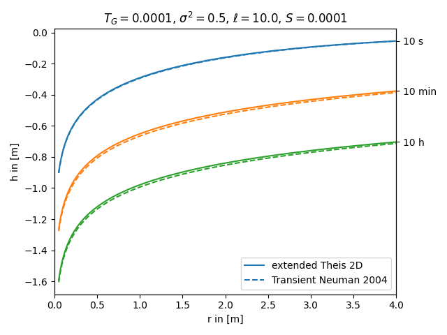
extended Theis 2D vs. transient solution for apparent transmissivity from Neuman

Both, the extended Theis and the Neuman solution, represent an effective transient drawdown in a heterogeneous aquifer. In both cases the heterogeneity is represented by two point statistics, characterized by mean, variance and length scale of the log transmissivity field. Therefore these approaches should lead to similar results.

References:

• Neuman 2004

• Zech et. al. 2016

import numpy as np
from matplotlib import pyplot as plt
from anaflow import ext_theis_2d, neuman2004


time_labels = ["10 s", "10 min", "10 h"]
time = [10, 600, 36000]  # 10s, 10min, 10h

rad = np.geomspace(0.05, 4)  # radius from the pumping well in [0, 4]

TG = 1e-4  # the geometric mean of the transmissivity
var = 0.5  # correlation length of the log-transmissivity
len_scale = 10.0  # variance of the log-transmissivity

S = 1e-4  # storativity
rate = -1e-4  # pumping rate

head1 = ext_theis_2d(time, rad, S, TG, var, len_scale, rate)
head2 = neuman2004(time, rad, S, TG, var, len_scale, rate)
time_ticks = []
for i, step in enumerate(time):
    label1 = "extended Theis 2D" if i == 0 else None
    label2 = "Transient Neuman 2004" if i == 0 else None
    plt.plot(rad, head1[i], label=label1, color="C" + str(i))
    plt.plot(rad, head2[i], label=label2, color="C" + str(i), linestyle="--")
    time_ticks.append(head1[i][-1])

plt.title(
    "$T_G={}$, $\sigma^2={}$, $\ell={}$, $S={}$".format(TG, var, len_scale, S)
)
plt.xlabel("r in [m]")
plt.ylabel("h in [m]")
plt.legend()
ylim = plt.gca().get_ylim()
plt.gca().set_xlim([0, rad[-1]])
ax2 = plt.gca().twinx()
ax2.set_yticks(time_ticks)
ax2.set_yticklabels(time_labels)
ax2.set_ylim(ylim)
plt.tight_layout()
plt.show()