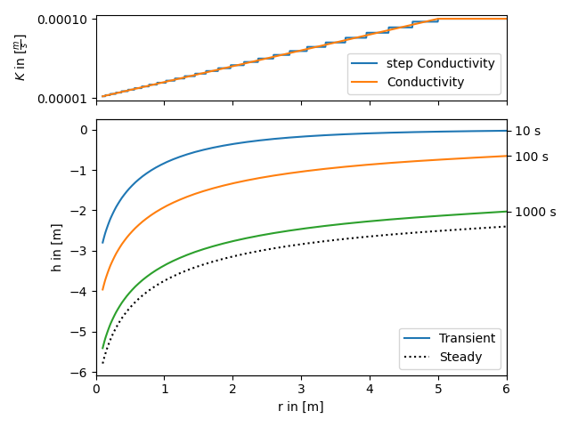
Self defined radial conductivity or transmissivity

All heterogeneous solutions of AnaFlow are derived by calculating an equivalent step function of a radial symmetric transmissivity resp. conductivity function.

The following code shows how to apply this workflow to a self defined transmissivity function. The function in use represents a linear transition from a local to a far field value of transmissivity within a given range.

The step function is calculated as the harmonic mean within given bounds, since the groundwater flow under a pumping condition is perpendicular to the different annular regions of transmissivity.

Reference: (not yet published)

import numpy as np
from matplotlib import pyplot as plt
import matplotlib.gridspec as gridspec
from anaflow import ext_grf, ext_grf_steady
from anaflow.tools import specialrange_cut, annular_hmean, step_f


def cond(rad, K_far, K_well, len_scale):
    """Conductivity with linear increase from K_well to K_far."""
    return np.minimum(np.abs(rad) / len_scale, 1.0) * (K_far - K_well) + K_well


time_labels = ["10 s", "100 s", "1000 s"]
time = [10, 100, 1000]
rad = np.geomspace(0.1, 6)

K_well = 1e-5
K_far = 1e-4
len_scale = 5.0
dim = 1.5

rate = -1e-4
S = 1e-4

cut_off = len_scale
parts = 30
r_well = 0.0
r_bound = 50.0

# calculate a disk-distribution of "trans" by calculating harmonic means
R_part = specialrange_cut(r_well, r_bound, parts, cut_off)
K_part = annular_hmean(
    cond, R_part, ann_dim=dim, K_far=K_far, K_well=K_well, len_scale=len_scale
)
S_part = np.full_like(K_part, S)
# calculate transient and steady heads
head1 = ext_grf(time, rad, S_part, K_part, R_part, dim=dim, rate=rate)
head2 = ext_grf_steady(
    rad,
    r_bound,
    cond,
    dim=dim,
    rate=-1e-4,
    K_far=K_far,
    K_well=K_well,
    len_scale=len_scale,
)

# plotting
gs = gridspec.GridSpec(2, 1, height_ratios=[1, 3])
ax1 = plt.subplot(gs[0])
ax2 = plt.subplot(gs[1], sharex=ax1)
time_ticks = []
for i, step in enumerate(time):
    label = "Transient" if i == 0 else None
    ax2.plot(rad, head1[i], label=label, color="C" + str(i))
    time_ticks.append(head1[i][-1])

ax2.plot(rad, head2, label="Steady", color="k", linestyle=":")

rad_lin = np.linspace(rad[0], rad[-1], 1000)
ax1.plot(rad_lin, step_f(rad_lin, R_part, K_part), label="step Conductivity")
ax1.plot(
    rad_lin, cond(rad_lin, K_far, K_well, len_scale), label="Conductivity"
)
ax1.set_yticks([K_well, K_far])
ax1.set_ylabel(r"$K$ in $[\frac{m}{s}]$")
plt.setp(ax1.get_xticklabels(), visible=False)
ax1.legend()
ax2.set_xlabel("r in [m]")
ax2.set_ylabel("h in [m]")
ax2.legend()
ax2.set_xlim([0, rad[-1]])
ax3 = ax2.twinx()
ax3.set_yticks(time_ticks)
ax3.set_yticklabels(time_labels)
ax3.set_ylim(ax2.get_ylim())

plt.tight_layout()
plt.show()