Tutorial 2: The extended Theis solution in 2D

We provide an extended theis solution, that incorporates the effectes of a heterogeneous transmissivity field on a pumping test.

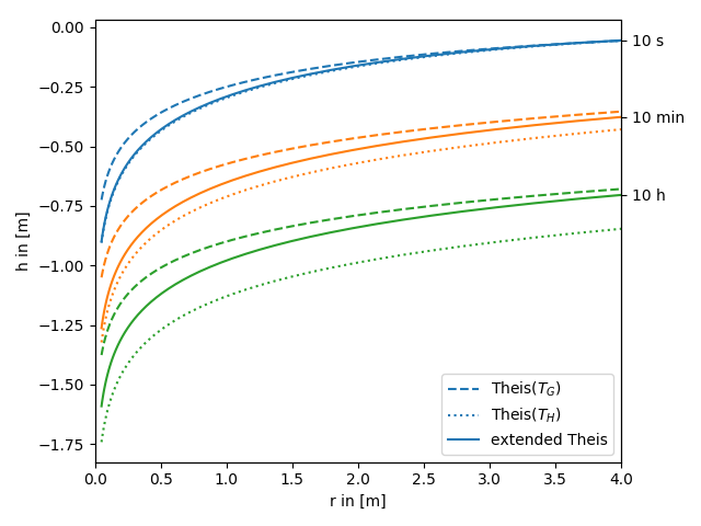
In the following this extended solution is compared to the standard theis solution for well flow. You can nicely see, that the extended solution represents a transition between the theis solutions for the geometric- and harmonic-mean transmissivity.

Reference: Zech et. al. 2016

import numpy as np
from matplotlib import pyplot as plt
from anaflow import theis, ext_theis_2d


time_labels = ["10 s", "10 min", "10 h"]
time = [10, 600, 36000]       # 10s, 10min, 10h
rad = np.geomspace(0.05, 4)   # radius from the pumping well in [0, 4]
var = 0.5                     # variance of the log-transmissivity
len_scale = 10.0              # correlation length of the log-transmissivity
TG = 1e-4                     # the geometric mean of the transmissivity
TH = TG * np.exp(-var / 2.0)  # the harmonic mean of the transmissivity
S = 1e-4                      # storativity
rate = -1e-4                  # pumping rate

head_TG = theis(time, rad, S, TG, rate)
head_TH = theis(time, rad, S, TH, rate)
head_ef = ext_theis_2d(time, rad, S, TG, var, len_scale, rate)
time_ticks=[]
for i, step in enumerate(time):
    label_TG = "Theis($T_G$)" if i == 0 else None
    label_TH = "Theis($T_H$)" if i == 0 else None
    label_ef = "extended Theis" if i == 0 else None
    plt.plot(rad, head_TG[i], label=label_TG, color="C"+str(i), linestyle="--")
    plt.plot(rad, head_TH[i], label=label_TH, color="C"+str(i), linestyle=":")
    plt.plot(rad, head_ef[i], label=label_ef, color="C"+str(i))
    time_ticks.append(head_ef[i][-1])

plt.xlabel("r in [m]")
plt.ylabel("h in [m]")
plt.legend()
ylim = plt.gca().get_ylim()
plt.gca().set_xlim([0, rad[-1]])
ax2 = plt.gca().twinx()
ax2.set_yticks(time_ticks)
ax2.set_yticklabels(time_labels)
ax2.set_ylim(ylim)
plt.tight_layout()
plt.show()