Tutorial 4: The extended Theis solution for truncated power laws

We provide an extended theis solution, that incorporates the effectes of a heterogeneous conductivity field following a truncated power law. In addition, it incorporates the assumptions of the general radial flow model and provides an arbitrary flow dimension.

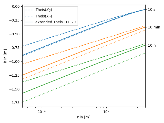
In the following this extended solution is compared to the standard theis solution for well flow. You can nicely see, that the extended solution represents a transition between the theis solutions for the well- and farfield-conductivity.

Reference: (not yet published)

import numpy as np
from matplotlib import pyplot as plt
from anaflow import theis, ext_theis_tpl


time_ticks = []
time_labels = ["10 s", "10 min", "10 h"]
time = [10, 600, 36000]      # 10s, 10min, 10h
rad = np.geomspace(0.05, 4)  # radial distance from the pumping well in [0, 4]
S = 1e-4                     # storage
KG = 1e-4                    # the geometric mean of the conductivity
len_scale = 20.0             # upper bound for the length scale
hurst = 0.5                  # hurst coefficient
var = 0.5                    # variance of the log-conductivity
rate = -1e-4                 # pumping rate
KH = KG * np.exp(-var / 2)   # the harmonic mean of the conductivity

head_KG = theis(time, rad, S, KG, rate)
head_KH = theis(time, rad, S, KH, rate)
head_ef = ext_theis_tpl(
    time=time,
    rad=rad,
    storage=S,
    cond_gmean=KG,
    len_scale=len_scale,
    hurst=hurst,
    var=var,
    rate=rate,
)
for i, step in enumerate(time):
    label_TG = "Theis($K_G$)" if i == 0 else None
    label_TH = "Theis($K_H$)" if i == 0 else None
    label_ef = "extended Theis TPL 2D" if i == 0 else None
    plt.plot(rad, head_KG[i], label=label_TG, color="C"+str(i), linestyle="--")
    plt.plot(rad, head_KH[i], label=label_TH, color="C"+str(i), linestyle=":")
    plt.plot(rad, head_ef[i], label=label_ef, color="C"+str(i))
    time_ticks.append(head_ef[i][-1])

plt.xscale("log")
plt.xlabel("r in [m]")
plt.ylabel("h in [m]")
plt.legend()
ylim = plt.gca().get_ylim()
plt.gca().set_xlim([rad[0], rad[-1]])
ax2 = plt.gca().twinx()
ax2.set_yticks(time_ticks)
ax2.set_yticklabels(time_labels)
ax2.set_ylim(ylim)
plt.tight_layout()
plt.show()