Tutorial 8: Advanced stuff
Beside the implementations of solutions form literatur, AnaFlow provides some advanced features to pimp the solutions for the groundwater flow equation.
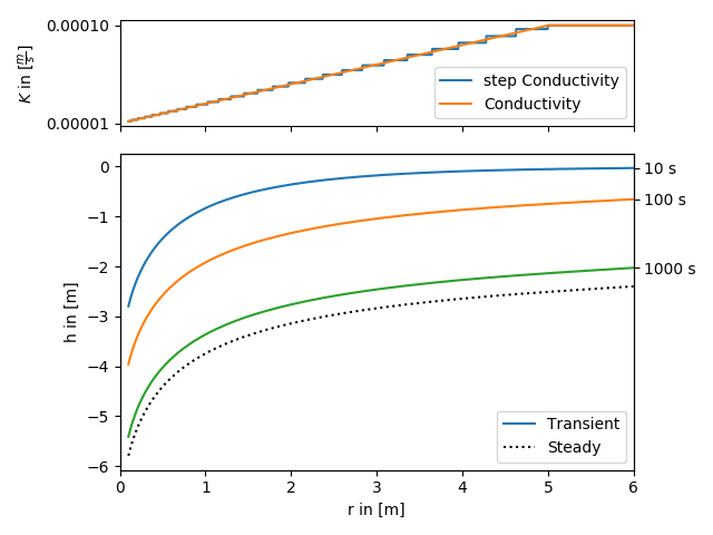
1. Self defined radial conductivity or transmissivity
All heterogeneous solutions of AnaFlow are derived by calculating an equivalent step function of a radial symmetric transmissivity resp. conductivity function.
The following code shows how to apply this workflow to a self defined transmissivity function. The function in use represents a linear transition from a local to a far field value of transmissivity within a given range.
The step function is calculated as the harmonic mean within given bounds, since the groundwater flow under a pumping condition is perpendicular to the different annular regions of transmissivity.
Reference: (not yet published)
import numpy as np
from matplotlib import pyplot as plt
import matplotlib.gridspec as gridspec
from anaflow import ext_grf, ext_grf_steady
from anaflow.tools import specialrange_cut, annular_hmean, step_f


def cond(rad, K_far, K_well, len_scale):
    """Conductivity with linear increase from K_well to K_far."""
    return np.minimum(np.abs(rad) / len_scale, 1.0) * (K_far - K_well) + K_well


time_labels = ["10 s", "100 s", "1000 s"]
time = [10, 100, 1000]
rad = np.geomspace(0.1, 6)
S = 1e-4
K_well = 1e-5
K_far = 1e-4
len_scale = 5.0
rate = -1e-4
dim = 1.5

cut_off = len_scale
parts = 30
r_well = 0.0
r_bound = 50.0

# calculate a disk-distribution of "trans" by calculating harmonic means
R_part = specialrange_cut(r_well, r_bound, parts, cut_off)
K_part = annular_hmean(cond, R_part, ann_dim=dim, K_far=K_far, K_well=K_well, len_scale=len_scale)
S_part = np.full_like(K_part, S)
# calculate transient and steady heads
head1 = ext_grf(time, rad, S_part, K_part, R_part, dim=dim, rate=rate)
head2 = ext_grf_steady(rad, r_bound, cond, dim=dim, rate=-1e-4, K_far=K_far, K_well=K_well, len_scale=len_scale)

# plotting
gs = gridspec.GridSpec(2, 1, height_ratios=[1, 3])
ax1 = plt.subplot(gs[0])
ax2 = plt.subplot(gs[1], sharex=ax1)
time_ticks=[]
for i, step in enumerate(time):
    label = "Transient" if i == 0 else None
    ax2.plot(rad, head1[i], label=label, color="C"+str(i))
    time_ticks.append(head1[i][-1])

ax2.plot(rad, head2, label="Steady", color="k", linestyle=":")

rad_lin = np.linspace(rad[0], rad[-1], 1000)
ax1.plot(rad_lin, step_f(rad_lin, R_part, K_part), label="step Conductivity")
ax1.plot(rad_lin, cond(rad_lin, K_far, K_well, len_scale), label="Conductivity")
ax1.set_yticks([K_well, K_far])
ax1.set_ylabel(r"$K$ in $[\frac{m}{s}]$")
plt.setp(ax1.get_xticklabels(), visible=False)
ax1.legend()
ax2.set_xlabel("r in [m]")
ax2.set_ylabel("h in [m]")
ax2.legend()
ax2.set_xlim([0, rad[-1]])
ax3 = ax2.twinx()
ax3.set_yticks(time_ticks)
ax3.set_yticklabels(time_labels)
ax3.set_ylim(ax2.get_ylim())

plt.tight_layout()
plt.show()
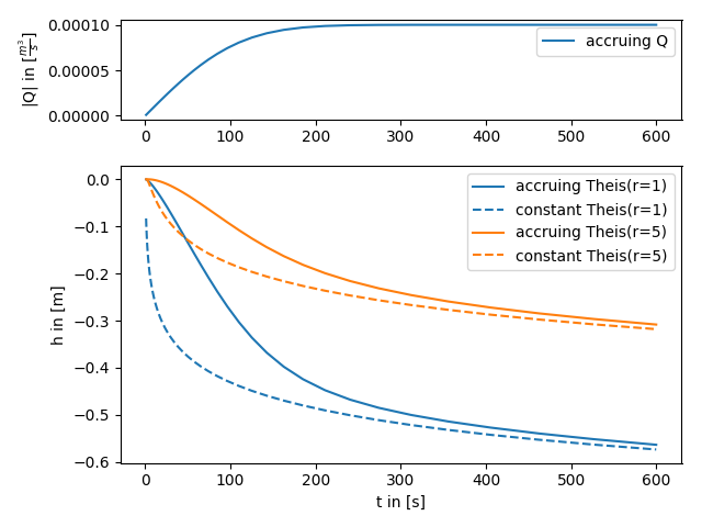
2. Accruing pumping rate
AnaFlow provides different representations for the pumping condition. One is an accruing pumping rate represented by the error function. This could be interpreted as that the water pump needs a certain time to reach its constant rate state.
import numpy as np
from scipy.special import erf
from matplotlib import pyplot as plt
import matplotlib.gridspec as gridspec
from anaflow import theis


time = np.geomspace(1, 600)
rad = [1, 5]

# Q(t) = Q * erf(t / a)
a = 120
lap_kwargs = {"cond": 4, "cond_kw": {"a": a}}
head1 = theis(
    time=time,
    rad=rad,
    storage=1e-4,
    transmissivity=1e-4,
    rate=-1e-4,
    lap_kwargs=lap_kwargs,
)
head2 = theis(
    time=time,
    rad=rad,
    storage=1e-4,
    transmissivity=1e-4,
    rate=-1e-4,
)
gs = gridspec.GridSpec(2, 1, height_ratios=[1, 3])
ax1 = plt.subplot(gs[0])
ax2 = plt.subplot(gs[1], sharex=ax1)

for i, step in enumerate(rad):
    ax2.plot(
        time,
        head1[:, i],
        color="C" + str(i),
        label="accruing Theis(r={})".format(step),
    )
    ax2.plot(
        time,
        head2[:, i],
        color="C" + str(i),
        label="constant Theis(r={})".format(step),
        linestyle="--"
    )
ax1.plot(time, 1e-4 * erf(time / a), label="accruing Q")
ax2.set_xlabel("t in [s]")
ax2.set_ylabel("h in [m]")
ax1.set_ylabel(r"|Q| in [$\frac{m^3}{s}$]")
ax1.legend()
ax2.legend()
plt.tight_layout()
plt.show()
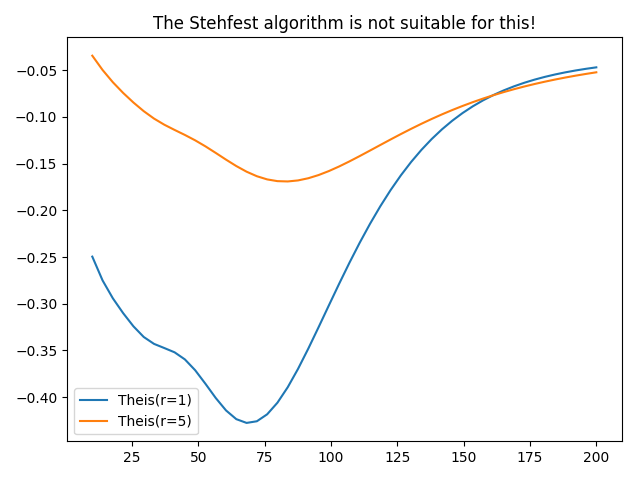
3. Interval pumping
Another case often discussed in literatur is interval pumping, where the pumping is just done in a certain time frame.
Unfortunatly the Stehfest algorithm is not suitable for this kind of solution, which is demonstrated in the following script.
import numpy as np
from matplotlib import pyplot as plt
from anaflow import theis


time = np.linspace(10, 200)
rad = [1, 5]

# Q(t) = Q * characteristic([0, T])
lap_kwargs = {"cond": 3, "cond_kw": {"a": 100}}
head = theis(
    time=time,
    rad=rad,
    storage=1e-4,
    transmissivity=1e-4,
    rate=-1e-4,
    lap_kwargs=lap_kwargs,
)

for i, step in enumerate(rad):
    plt.plot(time, head[:, i], label="Theis(r={})".format(step))

plt.title("The Stehfest algorithm is not suitable for this!")
plt.legend()
plt.tight_layout()
plt.show()