pentapy Tutorials

In the following you will find Tutorials on how to use pentapy.

Introduction: Solving a pentadiagonal system

Pentadiagonal systems arise in many areas of science and engineering, for example in solving differential equations with a finite difference sceme.

Theoretical Background

A pentadiagonal system is given by the equation: M\cdot X = Y, where M is a quadratic n\times n matrix given by:

M=\left(\begin{matrix}d_{1} & d_{1}^{\left(1\right)} & d_{1}^{\left(2\right)} & 0 & \cdots & \cdots & \cdots & \cdots & \cdots & 0\\
d_{2}^{\left(-1\right)} & d_{2} & d_{2}^{\left(1\right)} & d_{2}^{\left(2\right)} & 0 & \cdots & \cdots & \cdots & \cdots & 0\\
d_{3}^{\left(-2\right)} & d_{3}^{\left(-1\right)} & d_{3} & d_{3}^{\left(1\right)} & d_{3}^{\left(2\right)} & 0 & \cdots & \cdots & \cdots & 0\\
0 & d_{4}^{\left(-2\right)} & d_{4}^{\left(-1\right)} & d_{4} & d_{4}^{\left(1\right)} & d_{4}^{\left(2\right)} & 0 & \cdots & \cdots & 0\\
\vdots & \ddots & \ddots & \ddots & \ddots & \ddots & \ddots & \ddots & \ddots & \vdots\\
0 & \cdots & \cdots & \cdots & 0 & d_{n-2}^{\left(-2\right)} & d_{n-2}^{\left(-1\right)} & d_{n-2} & d_{n-2}^{\left(1\right)} & d_{n-2}^{\left(2\right)}\\
0 & \cdots & \cdots & \cdots & \cdots & 0 & d_{n-1}^{\left(-2\right)} & d_{n-1}^{\left(-1\right)} & d_{n-1} & d_{n-1}^{\left(1\right)}\\
0 & \cdots & \cdots & \cdots & \cdots & \cdots & 0 & d_{n}^{\left(-2\right)} & d_{n}^{\left(-1\right)} & d_{n}
\end{matrix}\right)

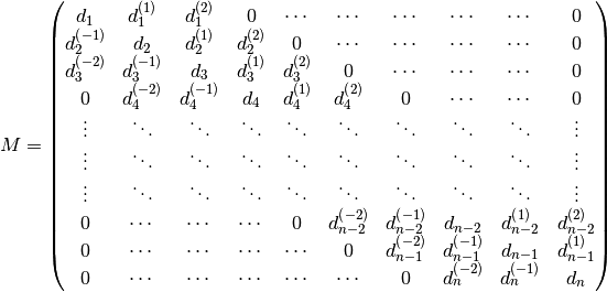
The aim is now, to solve this equation for X.

Memory efficient storage

To store a pentadiagonal matrix memory efficient, there are two options:

  1. row-wise storage:

M_{\mathrm{row}}=\left(\begin{matrix}d_{1}^{\left(2\right)} & d_{2}^{\left(2\right)} & d_{3}^{\left(2\right)} & \cdots & d_{n-2}^{\left(2\right)} & 0 & 0\\
d_{1}^{\left(1\right)} & d_{2}^{\left(1\right)} & d_{3}^{\left(1\right)} & \cdots & d_{n-2}^{\left(1\right)} & d_{n-1}^{\left(1\right)} & 0\\
d_{1} & d_{2} & d_{3} & \cdots & d_{n-2} & d_{n-1} & d_{n}\\
0 & d_{2}^{\left(-1\right)} & d_{3}^{\left(-1\right)} & \cdots & d_{n-2}^{\left(-1\right)} & d_{n-1}^{\left(-1\right)} & d_{n}^{\left(-1\right)}\\
0 & 0 & d_{3}^{\left(-2\right)} & \cdots & d_{n-2}^{\left(-2\right)} & d_{n-1}^{\left(-2\right)} & d_{n}^{\left(-2\right)}
\end{matrix}\right)

Here we see, that the numbering in the above given matrix was aiming at the row-wise storage. That means, the indices were taken from the row-indices of the entries.

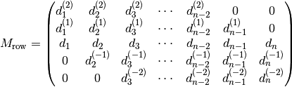
  1. column-wise storage:

M_{\mathrm{col}}=\left(\begin{matrix}0 & 0 & d_{1}^{\left(2\right)} & \cdots & d_{n-4}^{\left(2\right)} & d_{n-3}^{\left(2\right)} & d_{n-2}^{\left(2\right)}\\
0 & d_{1}^{\left(1\right)} & d_{2}^{\left(1\right)} & \cdots & d_{n-3}^{\left(1\right)} & d_{n-2}^{\left(1\right)} & d_{n-1}^{\left(1\right)}\\
d_{1} & d_{2} & d_{3} & \cdots & d_{n-2} & d_{n-1} & d_{n}\\
d_{2}^{\left(-1\right)} & d_{3}^{\left(-1\right)} & d_{4}^{\left(-1\right)} & \cdots & d_{n-1}^{\left(-1\right)} & d_{n}^{\left(-1\right)} & 0\\
d_{3}^{\left(-2\right)} & d_{4}^{\left(-2\right)} & d_{5}^{\left(-2\right)} & \cdots & d_{n}^{\left(-2\right)} & 0 & 0
\end{matrix}\right)

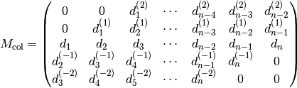
The numbering here is a bit confusing, but in the column-wise storage, all entries written in one column were in the same column in the original matrix.

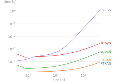
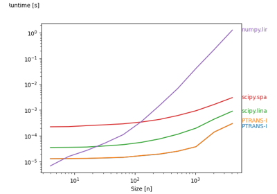
Solving the system using pentapy

To solve the system you can either provide M as a full matrix or as a flattened matrix in row-wise resp. col-wise flattened form.

If M is a full matrix, you call the following:

import pentapy as pp

M = ...  # your matrix
Y = ...  # your right hand side

X = pp.solve(M, Y)

If M is flattend in row-wise order you have to set the keyword argument is_flat=True:

import pentapy as pp

M = ...  # your flattened matrix
Y = ...  # your right hand side

X = pp.solve(M, Y, is_flat=True)

If you got a col-wise flattend matrix you have to set index_row_wise=False:

X = pp.solve(M, Y, is_flat=True, index_row_wise=False)

Tools

pentapy provides some tools to convert a pentadiagonal matrix.

diag_indices(n[, offset])

Get indices for the main or minor diagonals of a matrix.

shift_banded(mat[, up, low, col_to_row, copy])

Shift rows of a banded matrix.

create_banded(mat[, up, low, col_wise, dtype])

Create a banded matrix from a given quadratic Matrix.

create_full(mat[, up, low, col_wise])

Create a (n x n) Matrix from a given banded matrix.