Geometric example

A small example script showing the usage of the ‘geographic’ coordinates type for ordinary kriging on a sphere.

import numpy as np
from matplotlib import pyplot as plt

from pykrige.ok import OrdinaryKriging

# Make this example reproducible:
np.random.seed(89239413)

# Generate random data following a uniform spatial distribution
# of nodes and a uniform distribution of values in the interval
# [2.0, 5.5]:
N = 7
lon = 360.0 * np.random.random(N)
lat = 180.0 / np.pi * np.arcsin(2 * np.random.random(N) - 1)
z = 3.5 * np.random.rand(N) + 2.0

# Generate a regular grid with 60° longitude and 30° latitude steps:
grid_lon = np.linspace(0.0, 360.0, 7)
grid_lat = np.linspace(-90.0, 90.0, 7)

# Create ordinary kriging object:
OK = OrdinaryKriging(
    lon,
    lat,
    z,
    variogram_model="linear",
    verbose=False,
    enable_plotting=False,
    coordinates_type="geographic",
)

# Execute on grid:
z1, ss1 = OK.execute("grid", grid_lon, grid_lat)

# Create ordinary kriging object ignoring curvature:
OK = OrdinaryKriging(
    lon, lat, z, variogram_model="linear", verbose=False, enable_plotting=False
)

# Execute on grid:
z2, ss2 = OK.execute("grid", grid_lon, grid_lat)

Print data at equator (last longitude index will show periodicity):

print("Original data:")
print("Longitude:", lon.astype(int))
print("Latitude: ", lat.astype(int))
print("z:        ", np.array_str(z, precision=2))
print("\nKrige at 60° latitude:\n======================")
print("Longitude:", grid_lon)
print("Value:    ", np.array_str(z1[5, :], precision=2))
print("Sigma²:   ", np.array_str(ss1[5, :], precision=2))
print("\nIgnoring curvature:\n=====================")
print("Value:    ", np.array_str(z2[5, :], precision=2))
print("Sigma²:   ", np.array_str(ss2[5, :], precision=2))

Original data:
Longitude: [122 166  92 138  86 122 136]
Latitude:  [-46 -36 -25 -73 -25  50 -29]
z:         [2.75 3.36 2.24 3.07 3.37 5.25 2.82]

Krige at 60° latitude:
======================
Longitude: [  0.  60. 120. 180. 240. 300. 360.]
Value:     [5.29 5.11 5.27 5.17 5.35 5.63 5.29]
Sigma²:    [2.22 1.32 0.42 1.21 2.07 2.48 2.22]

Ignoring curvature:
=====================
Value:     [4.55 4.72 5.25 4.82 4.61 4.53 4.48]
Sigma²:    [3.79 2.   0.39 1.85 3.54 5.46 7.53]

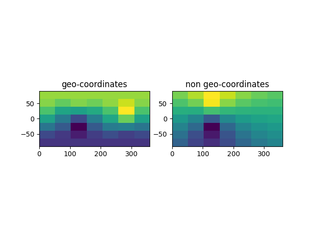
We can see that the data point at longitude 122, latitude 50 correctly dominates the kriged results, since it is the closest node in spherical distance metric, as longitude differences scale with cos(latitude). When kriging using longitude / latitude linearly, the value for grid points with longitude values further away as longitude is now incorrectly weighted equally as latitude.

fig, (ax1, ax2) = plt.subplots(1, 2)
ax1.imshow(z1, extent=[0, 360, -90, 90], origin="lower")
ax1.set_title("geo-coordinates")
ax2.imshow(z2, extent=[0, 360, -90, 90], origin="lower")
ax2.set_title("non geo-coordinates")
plt.show()