Note
Go to the end to download the full example code.
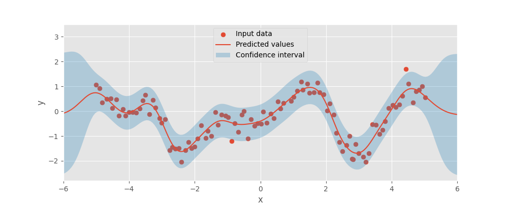
1D Kriging
An example of 1D kriging with PyKrige
import matplotlib.pyplot as plt
import numpy as np

from pykrige import OrdinaryKriging

plt.style.use("ggplot")

# fmt: off
# Data taken from
# https://blog.dominodatalab.com/fitting-gaussian-process-models-python/
X, y = np.array([
     [-5.01, 1.06], [-4.90, 0.92], [-4.82, 0.35], [-4.69, 0.49], [-4.56, 0.52],
     [-4.52, 0.12], [-4.39, 0.47], [-4.32,-0.19], [-4.19, 0.08], [-4.11,-0.19],
     [-4.00,-0.03], [-3.89,-0.03], [-3.78,-0.05], [-3.67, 0.10], [-3.59, 0.44],
     [-3.50, 0.66], [-3.39,-0.12], [-3.28, 0.45], [-3.20, 0.14], [-3.07,-0.28],
     [-3.01,-0.46], [-2.90,-0.32], [-2.77,-1.58], [-2.69,-1.44], [-2.60,-1.51],
     [-2.49,-1.50], [-2.41,-2.04], [-2.28,-1.57], [-2.19,-1.25], [-2.10,-1.50],
     [-2.00,-1.42], [-1.91,-1.10], [-1.80,-0.58], [-1.67,-1.08], [-1.61,-0.79],
     [-1.50,-1.00], [-1.37,-0.04], [-1.30,-0.54], [-1.19,-0.15], [-1.06,-0.18],
     [-0.98,-0.25], [-0.87,-1.20], [-0.78,-0.49], [-0.68,-0.83], [-0.57,-0.15],
     [-0.50, 0.00], [-0.38,-1.10], [-0.29,-0.32], [-0.18,-0.60], [-0.09,-0.49],
     [0.03 ,-0.50], [0.09 ,-0.02], [0.20 ,-0.47], [0.31 ,-0.11], [0.41 ,-0.28],
     [0.53 , 0.40], [0.61 , 0.11], [0.70 , 0.32], [0.94 , 0.42], [1.02 , 0.57],
     [1.13 , 0.82], [1.24 , 1.18], [1.30 , 0.86], [1.43 , 1.11], [1.50 , 0.74],
     [1.63 , 0.75], [1.74 , 1.15], [1.80 , 0.76], [1.93 , 0.68], [2.03 , 0.03],
     [2.12 , 0.31], [2.23 ,-0.14], [2.31 ,-0.88], [2.40 ,-1.25], [2.50 ,-1.62],
     [2.63 ,-1.37], [2.72 ,-0.99], [2.80 ,-1.92], [2.83 ,-1.94], [2.91 ,-1.32],
     [3.00 ,-1.69], [3.13 ,-1.84], [3.21 ,-2.05], [3.30 ,-1.69], [3.41 ,-0.53],
     [3.52 ,-0.55], [3.63 ,-0.92], [3.72 ,-0.76], [3.80 ,-0.41], [3.91 , 0.12],
     [4.04 , 0.25], [4.13 , 0.16], [4.24 , 0.26], [4.32 , 0.62], [4.44 , 1.69],
     [4.52 , 1.11], [4.65 , 0.36], [4.74 , 0.79], [4.84 , 0.87], [4.93 , 1.01],
     [5.02 , 0.55]
]).T
# fmt: on

X_pred = np.linspace(-6, 6, 200)

# pykrige doesn't support 1D data for now, only 2D or 3D
# adapting the 1D input to 2D
uk = OrdinaryKriging(X, np.zeros(X.shape), y, variogram_model="gaussian")

y_pred, y_std = uk.execute("grid", X_pred, np.array([0.0]))

y_pred = np.squeeze(y_pred)
y_std = np.squeeze(y_std)

fig, ax = plt.subplots(1, 1, figsize=(10, 4))
ax.scatter(X, y, s=40, label="Input data")


ax.plot(X_pred, y_pred, label="Predicted values")
ax.fill_between(
    X_pred,
    y_pred - 3 * y_std,
    y_pred + 3 * y_std,
    alpha=0.3,
    label="Confidence interval",
)
ax.legend(loc=9)
ax.set_xlabel("x")
ax.set_ylabel("y")
ax.set_xlim(-6, 6)
ax.set_ylim(-2.8, 3.5)
plt.show()
Total running time of the script: (0 minutes 0.100 seconds)