Tutorial 6: Comparison of different solutions

In the following we compare a set of different solutions of the groundwater flow equation.

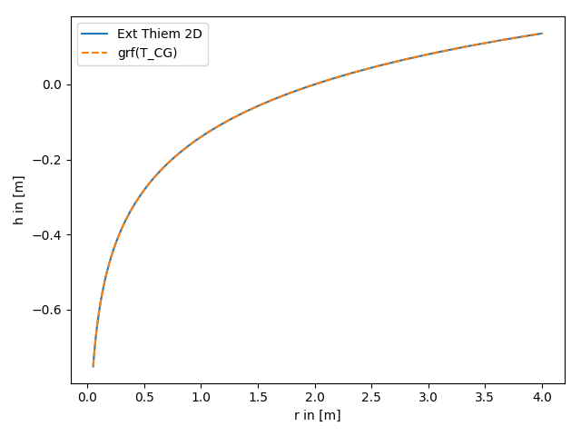
1. extended Thiem 2D vs. steady solution for coarse graining transmissivity

The extended Thiem 2D solutions is the analytical solution of the groundwater flow equation for the coarse graining transmissivity for pumping tests. Therefore the results should coincide.

References:

• Schneider & Attinger 2008
• Zech & Attinger 2016

import numpy as np
from matplotlib import pyplot as plt
from anaflow import ext_thiem_2d, ext_grf_steady
from anaflow.tools.coarse_graining import T_CG


rad = np.geomspace(0.05, 4)  # radius from the pumping well in [0, 4]
r_ref = 2.0                  # reference radius
var = 0.5                    # variance of the log-transmissivity
len_scale = 10.0             # correlation length of the log-transmissivity
TG = 1e-4                    # the geometric mean of the transmissivity
rate = -1e-4                 # pumping rate

head1 = ext_thiem_2d(rad, r_ref, TG, var, len_scale, rate)
head2 = ext_grf_steady(rad, r_ref, T_CG, rate=rate, trans_gmean=TG, var=var, len_scale=len_scale)

plt.plot(rad, head1, label="Ext Thiem 2D")
plt.plot(rad, head2, label="grf(T_CG)", linestyle="--")

plt.xlabel("r in [m]")
plt.ylabel("h in [m]")
plt.legend()
plt.tight_layout()
plt.show()

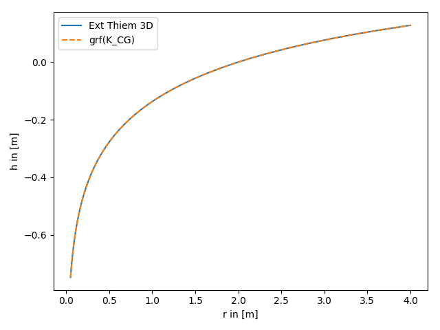
2. extended Thiem 3D vs. steady solution for coarse graining conductivity

The extended Thiem 3D solutions is the analytical solution of the groundwater flow equation for the coarse graining conductivity for pumping tests. Therefore the results should coincide.

Reference: Zech et. al. 2012

import numpy as np
from matplotlib import pyplot as plt
from anaflow import ext_thiem_3d, ext_grf_steady
from anaflow.tools.coarse_graining import K_CG


rad = np.geomspace(0.05, 4)  # radius from the pumping well in [0, 4]
r_ref = 2.0                  # reference radius
var = 0.5                    # variance of the log-transmissivity
len_scale = 10.0             # correlation length of the log-transmissivity
KG = 1e-4                    # the geometric mean of the transmissivity
anis = 0.7                   # aniso ratio
rate = -1e-4                 # pumping rate

head1 = ext_thiem_3d(rad, r_ref, KG, var, len_scale, anis, 1, rate)
head2 = ext_grf_steady(rad, r_ref, K_CG, rate=rate, cond_gmean=KG, var=var, len_scale=len_scale, anis=anis)

plt.plot(rad, head1, label="Ext Thiem 3D")
plt.plot(rad, head2, label="grf(K_CG)", linestyle="--")

plt.xlabel("r in [m]")
plt.ylabel("h in [m]")
plt.legend()
plt.tight_layout()
plt.show()

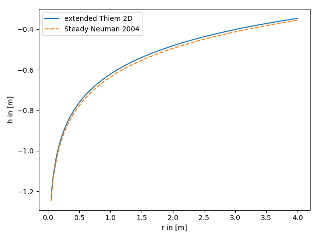
3. extended Thiem 2D vs. steady solution for apparent transmissivity from Neuman

Both, the extended Thiem and the Neuman solution, represent an effective steady drawdown in a heterogeneous aquifer. In both cases the heterogeneity is represented by two point statistics, characterized by mean, variance and length scale of the log transmissivity field. Therefore these approaches should lead to similar results.

References:

• Neuman 2004
• Zech & Attinger 2016

import numpy as np
from matplotlib import pyplot as plt
from anaflow import ext_thiem_2d, neuman2004_steady


rad = np.geomspace(0.05, 4)  # radius from the pumping well in [0, 4]
r_ref = 30.0                 # reference radius
var = 0.5                    # variance of the log-transmissivity
len_scale = 10.0             # correlation length of the log-transmissivity
TG = 1e-4                    # the geometric mean of the transmissivity
rate = -1e-4                 # pumping rate

head1 = ext_thiem_2d(rad, r_ref, TG, var, len_scale, rate)
head2 = neuman2004_steady(rad, r_ref, TG, var, len_scale, rate)

plt.plot(rad, head1, label="extended Thiem 2D")
plt.plot(rad, head2, label="Steady Neuman 2004", linestyle="--")

plt.xlabel("r in [m]")
plt.ylabel("h in [m]")
plt.legend()
plt.tight_layout()
plt.show()

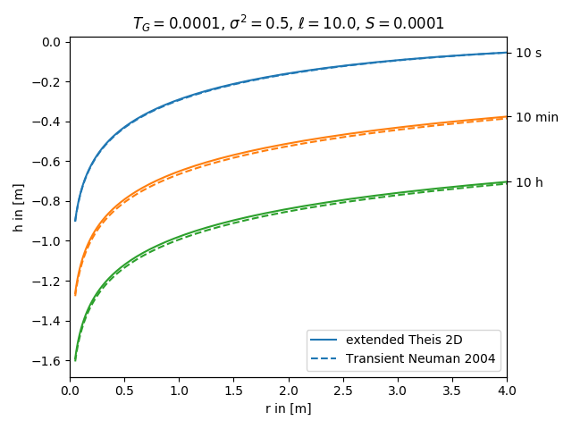
4. extended Theis 2D vs. transient solution for apparent transmissivity from Neuman

Both, the extended Theis and the Neuman solution, represent an effective transient drawdown in a heterogeneous aquifer. In both cases the heterogeneity is represented by two point statistics, characterized by mean, variance and length scale of the log transmissivity field. Therefore these approaches should lead to similar results.

References:

• Neuman 2004
• Zech et. al. 2016

import numpy as np
from matplotlib import pyplot as plt
from anaflow import ext_theis_2d, neuman2004


time_labels = ["10 s", "10 min", "10 h"]
time = [10, 600, 36000]      # 10s, 10min, 10h
rad = np.geomspace(0.05, 4)  # radius from the pumping well in [0, 4]
TG = 1e-4                    # the geometric mean of the transmissivity
var = 0.5                    # correlation length of the log-transmissivity
len_scale = 10.0             # variance of the log-transmissivity
S = 1e-4                     # storativity
rate = -1e-4                 # pumping rate

head1 = ext_theis_2d(time, rad, S, TG, var, len_scale, rate)
head2 = neuman2004(time, rad, S, TG, var, len_scale, rate)
time_ticks=[]
for i, step in enumerate(time):
    label1 = "extended Theis 2D" if i == 0 else None
    label2 = "Transient Neuman 2004" if i == 0 else None
    plt.plot(rad, head1[i], label=label1, color="C"+str(i))
    plt.plot(rad, head2[i], label=label2, color="C"+str(i), linestyle="--")
    time_ticks.append(head1[i][-1])

plt.title("$T_G={}$, $\sigma^2={}$, $\ell={}$, $S={}$".format(TG, var, len_scale, S))
plt.xlabel("r in [m]")
plt.ylabel("h in [m]")
plt.legend()
ylim = plt.gca().get_ylim()
plt.gca().set_xlim([0, rad[-1]])
ax2 = plt.gca().twinx()
ax2.set_yticks(time_ticks)
ax2.set_yticklabels(time_labels)
ax2.set_ylim(ylim)
plt.tight_layout()
plt.show()