GSTools Quickstart

GeoStatTools provides geostatistical tools for random field generation and variogram estimation based on many readily provided and even user-defined covariance models.
Installation
The package can be installed via pip. On Windows you can install WinPython to get Python and pip running.
pip install gstools
Spatial Random Field Generation
The core of this library is the generation of spatial random fields. These fields are generated using the randomisation method, described by Heße et al. 2014.
Examples
Gaussian Covariance Model
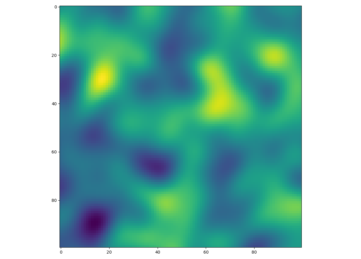
This is an example of how to generate a 2 dimensional spatial random field (SRF)
with a Gaussian covariance model.
from gstools import SRF, Gaussian
import matplotlib.pyplot as plt
# structured field with a size 100x100 and a grid-size of 1x1
x = y = range(100)
model = Gaussian(dim=2, var=1, len_scale=10)
srf = SRF(model)
field = srf((x, y), mesh_type='structured')
plt.imshow(field)
plt.show()
Truncated Power Law Model
GSTools also implements truncated power law variograms, which can be represented as a
superposition of scale dependant modes in form of standard variograms, which are truncated by
a lower-  and an upper length-scale
  .
.
This example shows the truncated power law (TPLStable) based on the
Stable covariance model and is given by
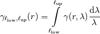
with Stable modes on each scale:
![\gamma(r,\lambda) &=
\sigma^2(\lambda)\cdot\left(1-
\exp\left[- \left(\frac{r}{\lambda}\right)^{\alpha}\right]
\right)\\
\sigma^2(\lambda) &= C\cdot\lambda^{2H}](_images/math/411c0961a08eb64bbff8f97954392676b2b12e82.png)
which gives Gaussian modes for alpha=2 or Exponential modes for alpha=1.
For  this results in:
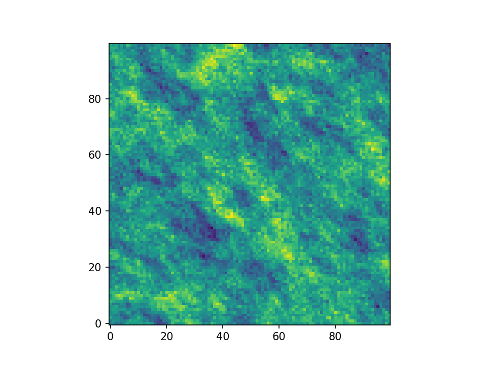
![\gamma_{\ell_{\mathrm{up}}}(r) &=
\sigma^2_{\ell_{\mathrm{up}}}\cdot\left(1-
\frac{2H}{\alpha} \cdot
E_{1+\frac{2H}{\alpha}}
\left[\left(\frac{r}{\ell_{\mathrm{up}}}\right)^{\alpha}\right]
\right) \\
\sigma^2_{\ell_{\mathrm{up}}} &=
C\cdot\frac{\ell_{\mathrm{up}}^{2H}}{2H}](_images/math/cf25b21cbeaf282001124c69aef6e1c51e7552fd.png)
import numpy as np
import matplotlib.pyplot as plt
from gstools import SRF, TPLStable
x = y = np.linspace(0, 100, 100)
model = TPLStable(
    dim=2,           # spatial dimension
    var=1,           # variance (C calculated internally, so that `var` is 1)
    len_low=0,       # lower truncation of the power law
    len_scale=10,    # length scale (a.k.a. range), len_up = len_low + len_scale
    nugget=0.1,      # nugget
    anis=0.5,        # anisotropy between main direction and transversal ones
    angles=np.pi/4,  # rotation angles
    alpha=1.5,       # shape parameter from the stable model
    hurst=0.7,       # hurst coefficient from the power law
)
srf = SRF(model, mean=1, mode_no=1000, seed=19970221, verbose=True)
field = srf((x, y), mesh_type='structured', force_moments=True)
# show the field in correct xy coordinates
plt.imshow(field.T, origin="lower")
plt.show()
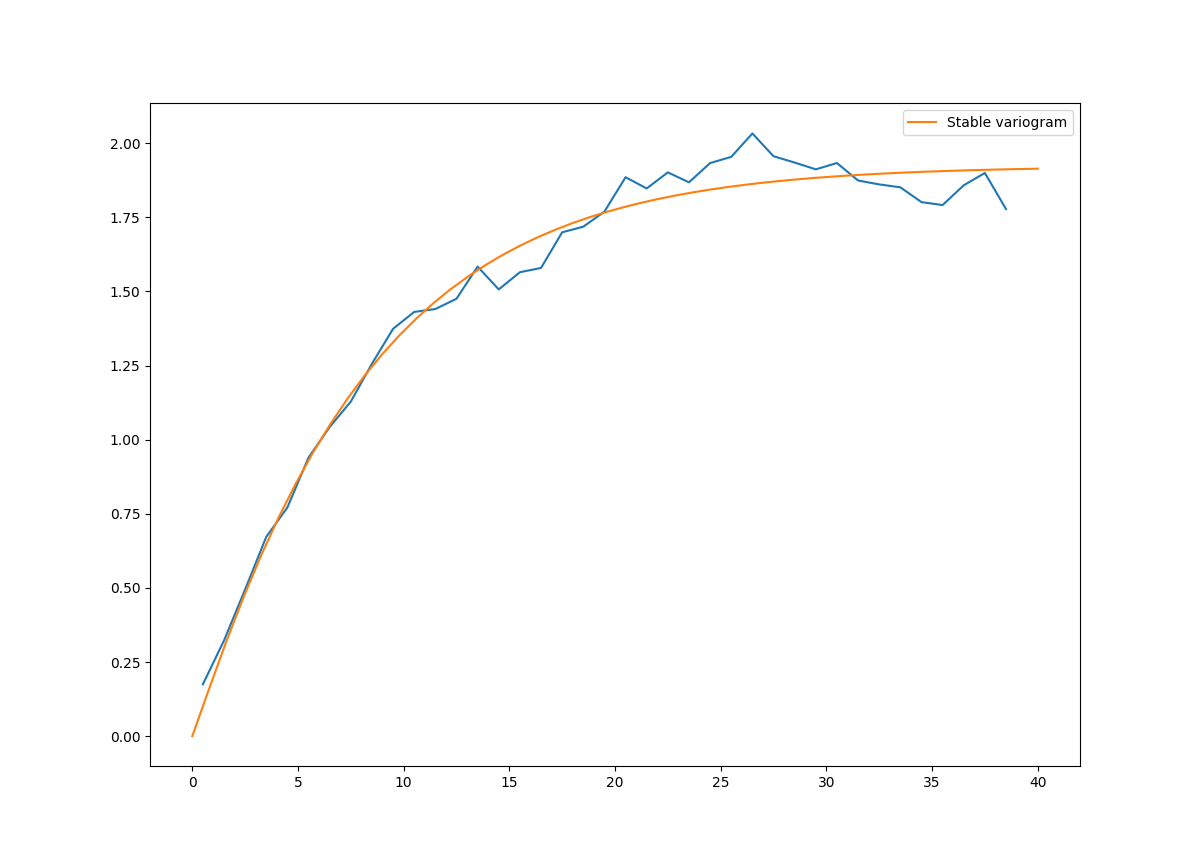
Estimating and fitting variograms
The spatial structure of a field can be analyzed with the variogram, which contains the same information as the covariance function.
All covariance models can be used to fit given variogram data by a simple interface.
Examples
This is an example of how to estimate the variogram of a 2 dimensional unstructured field and estimate the parameters of the covariance model again.
import numpy as np
from gstools import SRF, Exponential, Stable, vario_estimate_unstructured
from gstools.covmodel.plot import plot_variogram
import matplotlib.pyplot as plt
# generate a synthetic field with an exponential model
x = np.random.RandomState(19970221).rand(1000) * 100.
y = np.random.RandomState(20011012).rand(1000) * 100.
model = Exponential(dim=2, var=2, len_scale=8)
srf = SRF(model, mean=0, seed=19970221)
field = srf((x, y))
# estimate the variogram of the field with 40 bins
bins = np.arange(40)
bin_center, gamma = vario_estimate_unstructured((x, y), field, bins)
plt.plot(bin_center, gamma)
# fit the variogram with a stable model. (no nugget fitted)
fit_model = Stable(dim=2)
fit_model.fit_variogram(bin_center, gamma, nugget=False)
plot_variogram(fit_model, x_max=40)
# output
print(fit_model)
plt.show()
Which gives:
Stable(dim=2, var=1.92, len_scale=8.15, nugget=0.0, anis=[1.], angles=[0.], alpha=1.05)
User defined covariance models
One of the core-features of GSTools is the powerfull
CovModel
class, which allows to easy define covariance models by the user.
Examples
Here we reimplement the Gaussian covariance model by defining just the correlation function:
from gstools import CovModel
import numpy as np
# use CovModel as the base-class
class Gau(CovModel):
    def correlation(self, r):
        return np.exp(-(r/self.len_scale)**2)
And that’s it! With Gau you now have a fully working covariance model,
which you could use for field generation or variogram fitting as shown above.
VTK Export
After you have created a field, you may want to save it to file, so we provide
a handy VTK export routine (vtk_export):
from gstools import SRF, Gaussian, vtk_export
x = y = range(100)
model = Gaussian(dim=2, var=1, len_scale=10)
srf = SRF(model)
field = srf((x, y), mesh_type='structured')
vtk_export("field", (x, y), field, mesh_type='structured')
Which gives a RectilinearGrid VTK file field.vtr.