Higher Dimensions

GSTools provides experimental support for higher dimensions.

Anisotropy is the same as in lower dimensions:

• in n dimensions we need (n-1) anisotropy ratios

Rotation on the other hand is a bit more complex. With increasing dimensions more and more rotation angles are added in order to properply describe the rotated axes of anisotropy.

By design the first rotation angles coincide with the lower ones:

• 2D (rotation in x-y plane) -> 3D: first angle describes xy-plane rotation

• 3D (Tait-Bryan angles) -> 4D: first 3 angles coincide with Tait-Bryan angles

By increasing the dimension from n to (n+1), n angles are added:

• 2D (1 angle) -> 3D: 3 angles (2 added)

• 3D (3 angles) -> 4D: 6 angles (3 added)

the following list of rotation-planes are described by the list of angles in the model:

1. x-y plane

2. x-z plane

3. y-z plane

4. x-v plane

5. y-v plane

6. z-v plane

7. …

The rotation direction in these planes have alternating signs in order to match Tait-Bryan in 3D.

Let’s have a look at a 4D example, where we naively add a 4th dimension.

import matplotlib.pyplot as plt

import gstools as gs

dim = 4
size = 20
pos = [range(size)] * dim
model = gs.Exponential(dim=dim, len_scale=5)
srf = gs.SRF(model, seed=20170519)
field = srf.structured(pos)

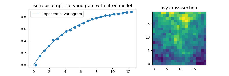
In order to “prove” correctness, we can calculate an empirical variogram of the generated field and fit our model to it.

bin_center, vario = gs.vario_estimate(
    pos, field, sampling_size=2000, mesh_type="structured"
)
model.fit_variogram(bin_center, vario)
print(model)

Exponential(dim=4, var=0.957, len_scale=4.79, nugget=2.77e-11)

As you can see, the estimated variance and length scale match our input quite well.

Let’s have a look at the fit and a x-y cross-section of the 4D field:

f, a = plt.subplots(1, 2, gridspec_kw={"width_ratios": [2, 1]}, figsize=[9, 3])
model.plot(x_max=max(bin_center), ax=a[0])
a[0].scatter(bin_center, vario)
a[1].imshow(field[:, :, 0, 0].T, origin="lower")
a[0].set_title("isotropic empirical variogram with fitted model")
a[1].set_title("x-y cross-section")
f.show()

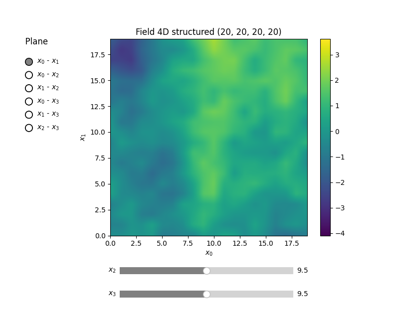
GSTools also provides plotting routines for higher dimensions. Fields are shown by 2D cross-sections, where other dimensions can be controlled via sliders.

srf.plot()