Anisotropy and Rotation

The internally used (semi-) variogram represents the isotropic case for the model. Nevertheless, you can provide anisotropy ratios by:

import gstools as gs

model = gs.Gaussian(dim=3, var=2.0, len_scale=10, anis=0.5)
print(model.anis)
print(model.len_scale_vec)

[1.  0.5]
[10. 10.  5.]

As you can see, we defined just one anisotropy-ratio and the second transversal direction was filled up with 1.. You can get the length-scales in each direction by the attribute CovModel.len_scale_vec. For full control you can set a list of anistropy ratios: anis=[0.5, 0.4].

Alternatively you can provide a list of length-scales:

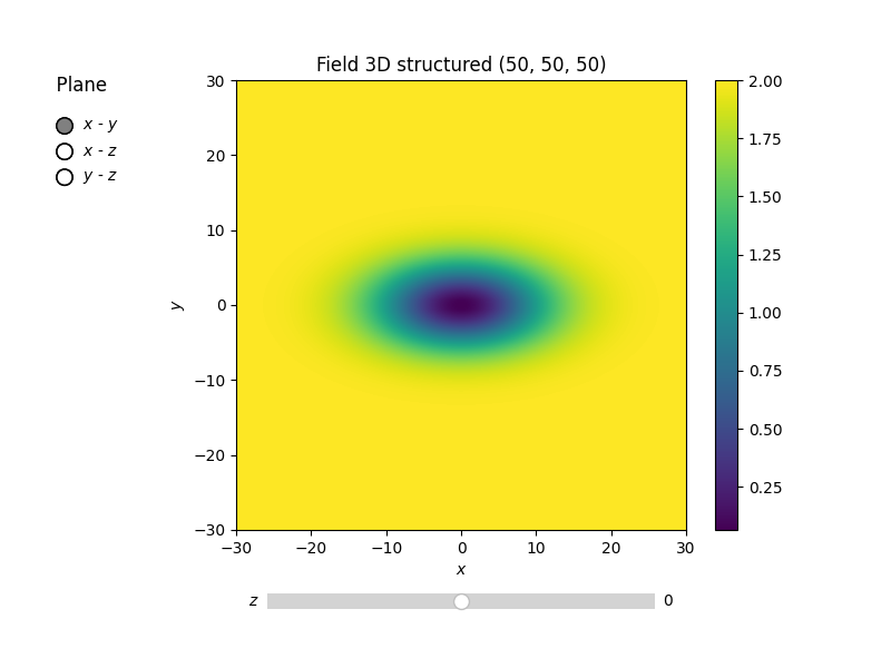
model = gs.Gaussian(dim=3, var=2.0, len_scale=[10, 5, 4])
model.plot("vario_spatial")
print("Anisotropy representations:")
print("Anis. ratios:", model.anis)
print("Main length scale", model.len_scale)
print("All length scales", model.len_scale_vec)

Anisotropy representations:
Anis. ratios: [0.5 0.4]
Main length scale 10.0
All length scales [10.  5.  4.]

Rotation Angles

The main directions of the field don’t have to coincide with the spatial directions \(x\), \(y\) and \(z\). Therefore you can provide rotation angles for the model:

model = gs.Gaussian(dim=3, var=2.0, len_scale=[10, 2], angles=2.5)
model.plot("vario_spatial")
print("Rotation angles", model.angles)

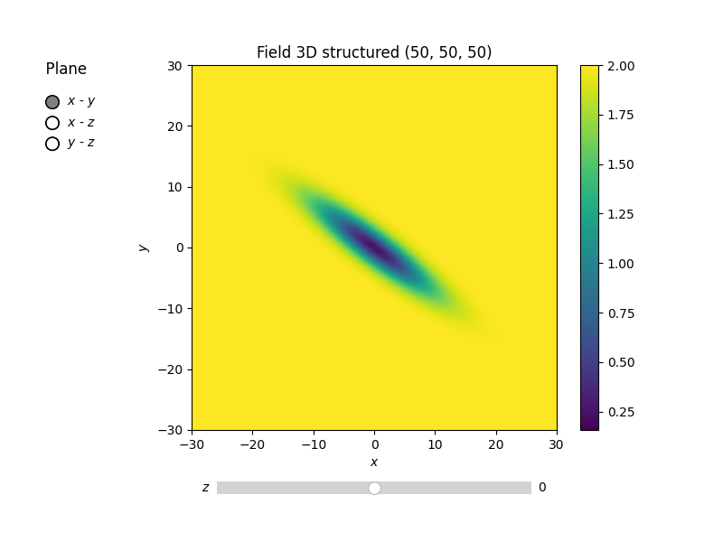
Rotation angles [2.5 0.  0. ]

Again, the angles were filled up with 0. to match the dimension and you could also provide a list of angles. The number of angles depends on the given dimension:

• in 1D: no rotation performable

• in 2D: given as rotation around z-axis

• in 3D: given by yaw, pitch, and roll (known as Tait–Bryan angles)

• in nD: See the random field example about higher dimensions