Plurigaussian Simulation
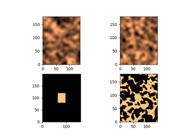
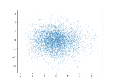
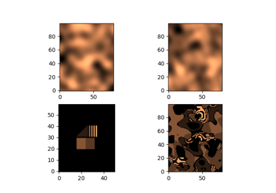
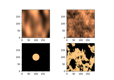
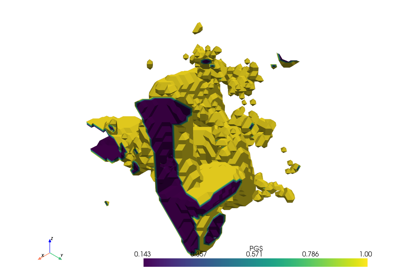
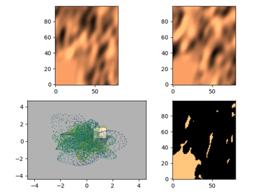
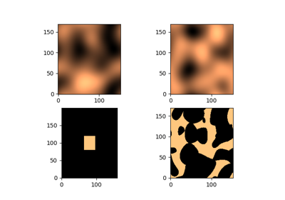
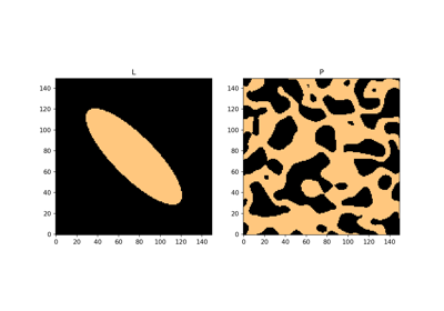
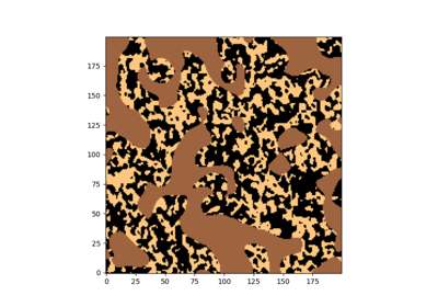
Plurigaussian simulation (PGS) is used to simulate correlated fields of categorical data, e.g. lithofacies, hydrofacies, soil types, or cementitious materials. In general, we define a categorical rule which dictates the relative frequency and connectivity of the phases present in the final realisation. We employ spatial random fields (SRFs) to map to this rule. This mapping determines the phase of a given point in the simulation domain. The definition of this rule limits how we can interact with it. For example, the rule may be defined spatially (e.g. as an image or array) or via a decision tree. Both forms will be explored in the following examples, highlighting their differences. Many PGS approaches constrain the number of input SRFs to match the dimensions of the simulation domain. This constraint stems from the implementation, not the method itself. With a spatial lithotype, we perform bigaussian and trigaussian simulations for two- and three-dimensional realisations, respectively. In contrast, the tree-based approach allows an arbitrary number of SRFs, yielding a fully plurigaussian simulation. This may sound more complicated than it is; we will clarify everything in the examples that follow.