Introductory example

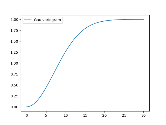
Let us start with a short example of a self defined model (Of course, we provide a lot of predefined models [See: gstools.covmodel], but they all work the same way). Therefore we reimplement the Gaussian covariance model by defining just the “normalized” correlation function:

import numpy as np

import gstools as gs


# use CovModel as the base-class
class Gau(gs.CovModel):
    def cor(self, h):
        return np.exp(-(h**2))

Here the parameter h stands for the normalized range r / len_scale. Now we can instantiate this model:

model = Gau(dim=2, var=2.0, len_scale=10)

To have a look at the variogram, let’s plot it:

model.plot()

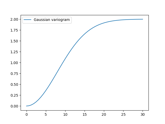
This is almost identical to the already provided Gaussian model. There, a scaling factor is implemented so the len_scale coincides with the integral scale:

gau_model = gs.Gaussian(dim=2, var=2.0, len_scale=10)
gau_model.plot()

Parameters

We already used some parameters, which every covariance models has. The basic ones are:

• dim : dimension of the model

• var : variance of the model (on top of the subscale variance)

• len_scale : length scale of the model

• nugget : nugget (subscale variance) of the model

These are the common parameters used to characterize a covariance model and are therefore used by every model in GSTools. You can also access and reset them:

print("old model:", model)
model.dim = 3
model.var = 1
model.len_scale = 15
model.nugget = 0.1
print("new model:", model)

old model: Gau(dim=2, var=2.0, len_scale=10.0, nugget=0.0)
new model: Gau(dim=3, var=1.0, len_scale=15.0, nugget=0.1)

Note

• The sill of the variogram is calculated by sill = variance + nugget So we treat the variance as everything above the nugget, which is sometimes called partial sill.

• A covariance model can also have additional parameters.