Roughness

The roughness describes the power-law behavior of a variogram at the origin ([Wu2016]):

\[\gamma(r) \sim c \cdot r^\alpha \quad (r \to 0)\]

The exponent \(\alpha\) is the roughness information, bounded by \(0 \le \alpha \le 2\). A value of 0 corresponds to a nugget effect and 2 is the smooth limit for random fields. You can access it via CovModel.roughness. On a log-log plot, the slope of the variogram near the origin approaches this value.

import numpy as np
import matplotlib.pyplot as plt

import gstools as gs

Variogram behavior near the origin

Compare variograms near the origin for models with different roughness.

models = [
    gs.Exponential(len_scale=1.0),
    gs.Gaussian(len_scale=1.0),
    gs.Stable(len_scale=1.0, alpha=0.7),
]

Use a small-lag grid and fit the slope on a log-log scale to estimate the roughness numerically.

r = np.logspace(-4, -1, 200)
fig, ax = plt.subplots()

for model in models:
    gamma = model.variogram(r)
    slope = np.polyfit(np.log(r[:20]), np.log(gamma[:20]), 1)[0]
    ax.loglog(
        r, gamma, label=rf"{model.name} ($\alpha={model.roughness:.2f}$)"
    )
    print(f"{model.name}: roughness={model.roughness:.2f}, fit={slope:.2f}")

ax.set_xlabel("r")
ax.set_ylabel(r"$\gamma(r)$")
ax.set_title("Variogram near the origin (log-log)")
ax.legend()

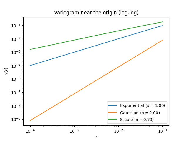
Exponential: roughness=1.00, fit=1.00
Gaussian: roughness=2.00, fit=2.00
Stable: roughness=0.70, fit=0.70

A nugget masks the power-law behavior at the origin, so roughness is 0.

nugget_model = gs.Gaussian(nugget=1.0)
print("Gaussian with nugget roughness:", nugget_model.roughness)

Gaussian with nugget roughness: 0.0

Roughness and random fields

From the theory of fractal stochastic processes (Mandelbrot and Van Ness 1968) ([Mandelbrot1968]), the roughness can be interpreted as:

1. Persistent (\(1 < \alpha \le 2\)): smooth behavior, slowly increasing variogram, long memory (e.g. Gaussian-like).

2. Antipersistent (\(0 < \alpha < 1\)): rough behavior, steep variogram near the origin, short memory.

3. No memory (\(\alpha = 1\)): linear slope at the origin (Exponential).

The Integral model lets us control the roughness with its parameter nu. For this model, the roughness is given by \(\alpha = \min(2, \nu)\).

Set up a common grid and plotting scales so the realizations are comparable.

sep = 100  # separation point (mid field)
ext = 10  # field extend
imext = 2 * [0, ext]
x = y = np.linspace(0, ext, 2 * sep + 1)
xm = np.linspace(0, 5, 1001)
vmin, vmax = -3, 3

Create Integral models with the same integral scale but different roughness.

rough = [0.1, 1, 10]
mod = [gs.Integral(dim=2, integral_scale=1, nu=nu) for nu in rough]

Note

Rough fields require a higher mode_no so the randomization method samples the high-frequency part of the spectrum sufficiently well.

Generate random field realizations with a shared seed for fair comparison.

srf = []
for m in mod:
    mode_no = int(1000 / m.roughness)  # increase mode_no for rough fields
    s = gs.SRF(m, seed=20110101, mode_no=mode_no)
    s.structured((x, y))
    srf.append(s)

Plot variograms, fields, and cross sections column-wise by roughness.

fig, axes = plt.subplots(3, 3, figsize=(10, 10))
for i in range(3):
    label = rf"$\alpha(\gamma)={mod[i].roughness:.2f}$"
    axes[0, i].plot(xm, mod[i].variogram(xm), label=label)
    axes[0, i].legend(loc="lower right")
    axes[0, i].set_ylim([-0.05, 1.05])
    axes[0, i].set_xlim([-0.25, 5.25])
    axes[0, i].grid()
    axes[1, i].imshow(
        srf[i].field.T,
        origin="lower",
        interpolation="bicubic",
        vmin=vmin,
        vmax=vmax,
        extent=imext,
    )
    axes[1, i].axhline(y=5, color="k")
    axes[2, i].plot(x, srf[i].field[:, sep])
    axes[2, i].set_ylim([vmin, vmax])
    axes[2, i].set_xlim([0, ext])
    axes[2, i].grid()

axes[0, 0].set_ylabel(r"$\gamma$")
axes[1, 0].set_ylabel(r"$y$")
axes[2, 0].set_ylabel(r"$f$")
axes[2, 0].set_xlabel(r"$x$")
axes[2, 1].set_xlabel(r"$x$")
axes[2, 2].set_xlabel(r"$x$")
fig.tight_layout()

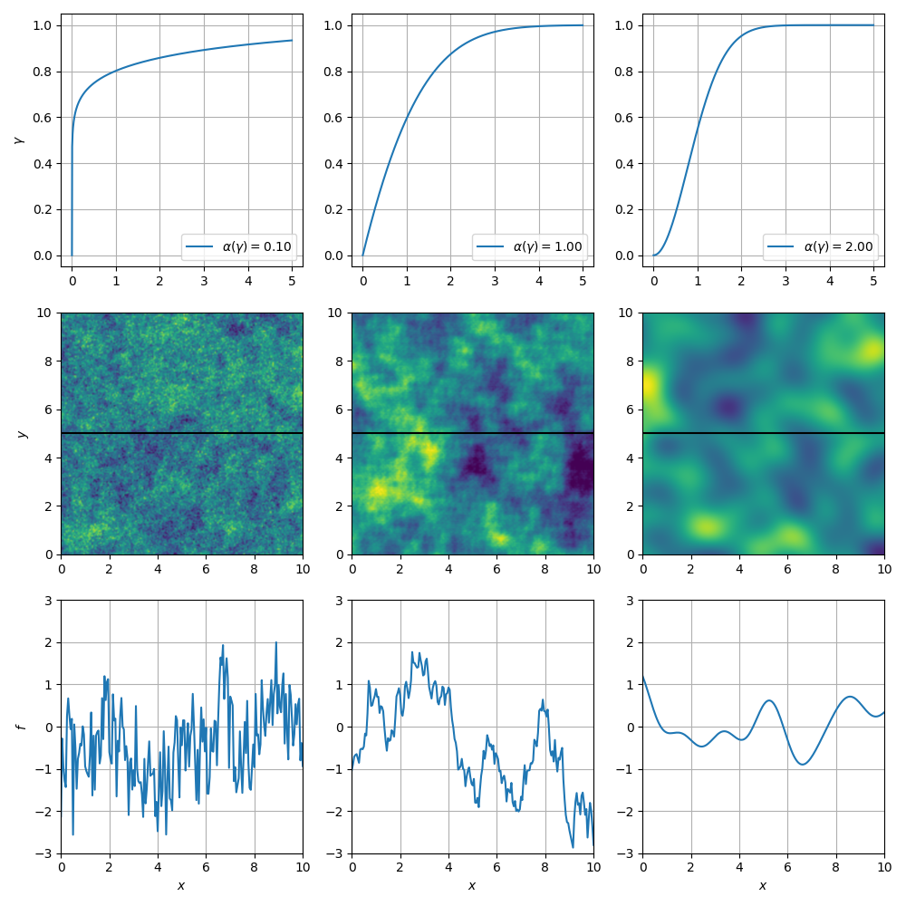
Illustration of the impact of the roughness information on spatial random fields. Each column shows the variogram on top, a single field realization in the middle and the highlighted cross section of the field on the bottom. The left column shows a very rough (antipersistent) field with a steep increase of the variogram at the origin, the middle column shows an Exponential like variogram with a linear slope at the origin resulting in a less rough (no memory) field and the right column shows a Gaussian like variogram together with a very smooth (persistent) field. All variograms have the same integral scale and x- and y-axis are given in multiples of the integral scale.

References

[Wu2016]

Wu, W.-Y., and C. Y. Lim. 2016. “ESTIMATION OF SMOOTHNESS OF A STATIONARY GAUSSIAN RANDOM FIELD.” Statistica Sinica 26 (4): 1729-1745. https://doi.org/10.5705/ss.202014.0109.

[Mandelbrot1968]

Mandelbrot, B. B., and J. W. Van Ness. 1968. “Fractional Brownian Motions, Fractional Noises and Applications.” SIAM Review 10 (4): 422-437. https://doi.org/10.1137/1010093.