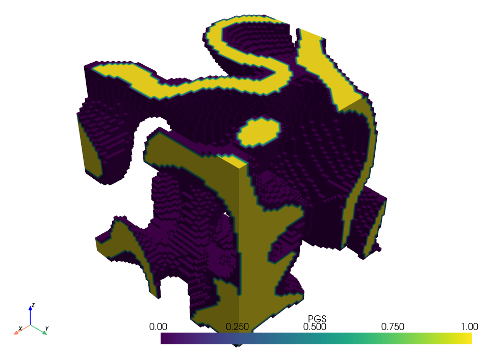
Three dimensional PGS through decision trees

Let’s apply the decision tree approach to three dimensional PGS

import numpy as np

import gstools as gs

dim = 3

# no. of cells in all dimensions
N = [60] * dim

x = np.arange(N[0])
y = np.arange(N[1])
z = np.arange(N[2])

As we want to generate a three dimensional field, we generate three spatial random fields (SRF) as our input. In this example, the number of fields is equal to the number of dimensions, but as before, this is not a requirement.

model = gs.Gaussian(dim=dim, var=1, len_scale=[15, 15, 15])
srf = gs.SRF(model)
field1 = srf.structured([x, y, z], seed=20277519)
field2 = srf.structured([x, y, z], seed=19727221)
field3 = srf.structured([x, y, z], seed=21145612)

The decision tree will now utilise an ellipsoid as the decision boundary, having a similar structure as the ellipse in the previous example.

def ellipsoid(data, key1, key2, key3, c1, c2, c3, s1, s2, s3):
    return ((data[key1] - c1) / s1) ** 2 + ((data[key2] - c2) / s2) ** 2 + (
        (data[key3] - c3) / s3
    ) ** 2 <= 1


config = {
    "root": {
        "type": "decision",
        "func": ellipsoid,
        "args": {
            "key1": "Z1",
            "key2": "Z2",
            "key3": "Z3",
            "c1": 0,
            "c2": 0,
            "c3": 0,
            "s1": 3,
            "s2": 1,
            "s3": 0.4,
        },
        "yes_branch": "phase1",
        "no_branch": "phase0",
    },
    "phase0": {"type": "leaf", "action": 0},
    "phase1": {"type": "leaf", "action": 1},
}

As before, we initialise the PGS process, generate P, and plot to visualise the results

import pyvista as pv

pgs = gs.PGS(dim, [field1, field2, field3])
P = pgs(tree=config)

grid = pv.ImageData(dimensions=N)
grid.point_data["PGS"] = P.reshape(-1)
grid.threshold(0.5, scalars="PGS").plot()