From bigaussian to plurigaussian simulation

In many PGS implementations, the dimensions of the simulation domain often matches the number of fields that are supplied. However, this is not a requirement of the PGS algorithm. In fact, it is possible to use multiple spatial random fields in PGS, which can be useful for more complex lithotype definitions. In this example, we will demonstrate how to use multiple SRFs in PGS. In GSTools, this is done by utilising the tree based architecture.

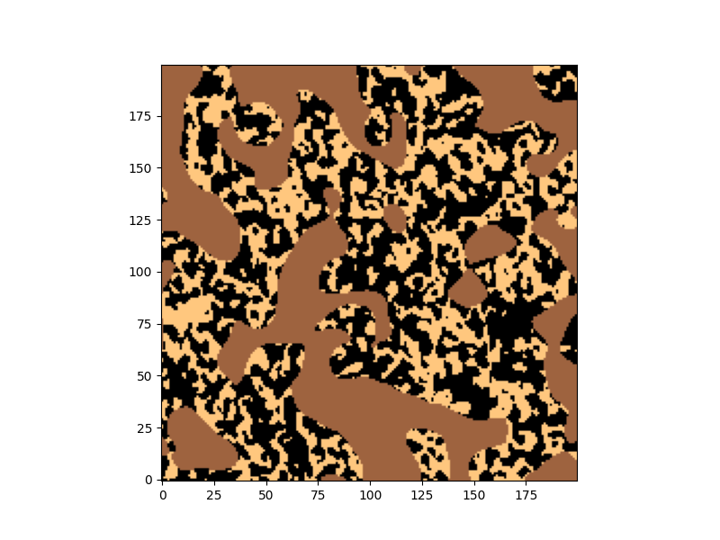
Typically, PGS in two dimensions is carried out as a bigaussian simulation, where two random fields are used. Here, we will employ four. We begin by setting up the simulation domain and generating the necessary random fields, where the length scales of two of the fields are much larger than the other two.

import matplotlib.pyplot as plt
import numpy as np

import gstools as gs

dim = 2

N = [200, 200]

x = np.arange(N[0])
y = np.arange(N[1])

model = gs.Gaussian(dim=dim, var=1, len_scale=15)
srf = gs.SRF(model)
field1 = srf.structured([x, y], seed=201519)
field2 = srf.structured([x, y], seed=199221)
model = gs.Gaussian(dim=dim, var=1, len_scale=3)
srf = gs.SRF(model)
field3 = srf.structured([x, y], seed=1345134)
field4 = srf.structured([x, y], seed=1351455)

As in the previous example, an ellipse is used as the decision boundary.

def ellipse(data, key1, key2, c1, c2, s1, s2, angle=0):
    x, y = data[key1] - c1, data[key2] - c2

    if angle:
        theta = np.deg2rad(angle)
        c, s = np.cos(theta), np.sin(theta)
        x, y = x * c + y * s, -x * s + y * c

    return (x / s1) ** 2 + (y / s2) ** 2 <= 1

The configuration dictionary for the decision tree is defined as before, but this time we pass the additional keys Z3 and Z4, which refer to the additional fields field3 and field4. The decision tree is structured in a way that the first decision node is based on the first two fields, and the second decision node is based on the last two fields.

config = {
    "root": {
        "type": "decision",
        "func": ellipse,
        "args": {
            "key1": "Z1",
            "key2": "Z2",
            "c1": 0.7,
            "c2": 0.7,
            "s1": 1.3,
            "s2": 1.3,
        },
        "yes_branch": "phase1",
        "no_branch": "node1",
    },
    "node1": {
        "type": "decision",
        "func": ellipse,
        "args": {
            "key1": "Z3",
            "key2": "Z4",
            "c1": -0.7,
            "c2": -0.7,
            "s1": 1.3,
            "s2": 1.3,
            "angle": 30,
        },
        "yes_branch": "phase2",
        "no_branch": "phase0",
    },
    "phase2": {"type": "leaf", "action": 2},
    "phase1": {"type": "leaf", "action": 1},
    "phase0": {"type": "leaf", "action": 0},
}

Next, we create the PGS object, passing in all four fields, and generate the plurigaussian field P

pgs = gs.PGS(dim, [field1, field2, field3, field4])

P = pgs(tree=config)

Finally, we plot P

NB: In the current implementation, the calculation of the equivalent spatial lithotype L is not supported for multiple fields

plt.figure(figsize=(8, 6))
plt.imshow(P, cmap="copper", origin="lower")