gstools.covmodel.tpl_models¶

GStools subpackage providing truncated power law covariance models.

The following classes and functions are provided

`TPLGaussian`([dim, var, len_scale, nugget, …])	Truncated-Power-Law with Gaussian modes.
`TPLExponential`([dim, var, len_scale, …])	Truncated-Power-Law with Exponential modes.
`TPLStable`([dim, var, len_scale, nugget, …])	Truncated-Power-Law with Stable modes.

class gstools.covmodel.tpl_models.TPLGaussian(dim=3, var=1.0, len_scale=1.0, nugget=0.0, anis=1.0, angles=0.0, integral_scale=None, var_raw=None, hankel_kw=None, **opt_arg)[source]¶

Bases: gstools.covmodel.base.CovModel

Truncated-Power-Law with Gaussian modes.

Notes

The truncated power law is given by a superposition of scale-dependent variograms:

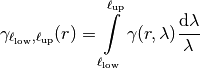
$\gamma_{\ell_{\mathrm{low}},\ell_{\mathrm{up}}}(r) = \intop_{\ell_{\mathrm{low}}}^{\ell_{\mathrm{up}}} \gamma(r,\lambda) \frac{\rm d \lambda}{\lambda}$

with Gaussian modes on each scale:

$\gamma(r,\lambda) &= \sigma^2(\lambda)\cdot\left(1- \exp\left[- \left(\frac{r}{\lambda}\right)^{2}\right] \right)\\ \sigma^2(\lambda) &= C\cdot\lambda^{2H}$

This results in:

$\gamma_{\ell_{\mathrm{low}},\ell_{\mathrm{up}}}(r) &= \sigma^2_{\ell_{\mathrm{low}},\ell_{\mathrm{up}}}\cdot\left(1- H \cdot \frac{\ell_{\mathrm{up}}^{2H} \cdot E_{1+H} \left[\left(\frac{r}{\ell_{\mathrm{up}}}\right)^{2}\right] - \ell_{\mathrm{low}}^{2H} \cdot E_{1+H} \left[\left(\frac{r}{\ell_{\mathrm{low}}}\right)^{2}\right]} {\ell_{\mathrm{up}}^{2H}-\ell_{\mathrm{low}}^{2H}} \right) \\ \sigma^2_{\ell_{\mathrm{low}},\ell_{\mathrm{up}}} &= \frac{C\cdot\left(\ell_{\mathrm{up}}^{2H} -\ell_{\mathrm{low}}^{2H}\right)}{2H}$

The “length scale” of this model is equivalent by the integration range:

$\ell = \ell_{\mathrm{up}} -\ell_{\mathrm{low}}$

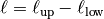
If you want to define an upper scale truncation, you should set len_low and len_scale accordingly.

The following Parameters occure:

$C>0$ : The scaling factor from the Power-Law. This parameter will be calculated internally by the given variance. You can access C directly by model.var_raw

$0<H<1$ : The hurst coefficient (model.hurst)

$\ell_{\mathrm{low}}\geq 0$ : The lower length scale truncation of the model (model.len_low)

$\ell_{\mathrm{up}}\geq 0$ : The upper length scale truncation of the model (model.len_up)

This will be calculated internally by:

len_up = len_low + len_scale

That means, that the len_scale in this model actually represents the integration range for the truncated power law.

$E_s(x)$ is the exponential integral.

Other Parameters:
	opt_arg – The following parameters are covered by these keyword arguments hurst (`float`, optional) – Hurst coefficient of the power law. Standard range: `(0, 1)`. Default: `0.5` len_low** (`float`, optional) – The lower length scale truncation of the model. Standard range: `[0, 1000]`. Default: `0.0` .
Parameters:	dim (`int`, optional) – dimension of the model. Default: `3` var (`float`, optional) – variance of the model (the nugget is not included in “this” variance) Default: `1.0` len_scale (`float` or `list`, optional) – length scale of the model. If a single value is given, the same length-scale will be used for every direction. If multiple values (for main and transversal directions) are given, anis will be recalculated accordingly. Default: `1.0` nugget (`float`, optional) – nugget of the model. Default: `0.0` anis (`float` or `list`, optional) – anisotropy ratios in the transversal directions [y, z]. Default: `1.0` angles (`float` or `list`, optional) – angles of rotation: in 2D: given as rotation around z-axis in 3D: given by yaw, pitch, and roll (known as Tait–Bryan angles) Default: `0.0` integral_scale (`float` or `list` or `None`, optional) – If given, `len_scale` will be ignored and recalculated, so that the integral scale of the model matches the given one. Default: `None` var_raw (`float` or `None`, optional) – raw variance of the model which will be multiplied with `CovModel.var_factor` to result in the actual variance. If given, `var` will be ignored. (This is just for models that override `CovModel.var_factor`) Default: `None` hankel_kw (`dict` or `None`, optional) – Modify the init-arguments of `hankel.SymmetricFourierTransform` used for the spectrum calculation. Use with caution (Better: Don’t!). `None` is equivalent to `{"a": -1, "b": 1, "N": 1000, "h": 0.001}`.
Attributes:	`angles` `numpy.ndarray`: Rotation angles (in rad) of the model. `anis` `numpy.ndarray`: The anisotropy factors of the model. `arg` `list` of `str`: Names of all arguments. `arg_bounds` `dict`: Bounds for all parameters. `dim` `int`: The dimension of the model. `dist_func` `tuple` of `callable`: pdf, cdf and ppf. `do_rotation` `bool`: State if a rotation is performed. `hankel_kw` `dict`: `hankel.SymmetricFourierTransform` kwargs. `has_cdf` `bool`: State if a cdf is defined by the user. `has_ppf` `bool`: State if a ppf is defined by the user. `integral_scale` `float`: The main integral scale of the model. `integral_scale_vec` `numpy.ndarray`: The integral scales in each direction. `len_scale` `float`: The main length scale of the model. `len_scale_bounds` `list`: Bounds for the lenght scale. `len_scale_vec` `numpy.ndarray`: The length scales in each direction. `len_up` `float`: Upper length scale truncation of the model. `name` `str`: The name of the CovModel class. `nugget` `float`: The nugget of the model. `nugget_bounds` `list`: Bounds for the nugget. `opt_arg` `list` of `str`: Names of the optional arguments. `opt_arg_bounds` `dict`: Bounds for the optional arguments. `pykrige_angle` 2D rotation angle for pykrige. `pykrige_angle_x` 3D rotation angle around x for pykrige. `pykrige_angle_y` 3D rotation angle around y for pykrige. `pykrige_angle_z` 3D rotation angle around z for pykrige. `pykrige_anis` 2D anisotropy ratio for pykrige. `pykrige_anis_y` 3D anisotropy ratio in y direction for pykrige. `pykrige_anis_z` 3D anisotropy ratio in z direction for pykrige. `pykrige_kwargs` Keyword arguments for pykrige routines. `sill` `float`: The sill of the variogram. `var` `float`: The variance of the model. `var_bounds` `list`: Bounds for the variance. `var_raw` `float`: The raw variance of the model without factor.

Methods

`calc_integral_scale`()	Calculate the integral scale of the isotrope model.
`check_arg_bounds`()	Check arguments to be within the given bounds.
`check_opt_arg`()	Run checks for the optional arguments.
`cor_spatial`(pos)	Spatial correlation respecting anisotropy and rotation.
`correlation`(r)	Truncated-Power-Law with Gaussian modes - correlation function.
`cov_nugget`(r)	Covariance of the model respecting the nugget at r=0.
`cov_spatial`(pos)	Spatial covariance respecting anisotropy and rotation.
`covariance`(r)	Covariance of the model.
`default_arg_bounds`()	Provide default boundaries for arguments.
`default_opt_arg`()	Defaults for the optional arguments.
`default_opt_arg_bounds`()	Defaults for boundaries of the optional arguments.
`fit_variogram`(x_data, y_data[, maxfev])	Fiting the isotropic variogram-model to given data.
`fix_dim`()	Set a fix dimension for the model.
`ln_spectral_rad_pdf`(r)	Log radial spectral density of the model.
`percentile_scale`([per])	Calculate the percentile scale of the isotrope model.
`plot`([func])	Plot a function of a the CovModel.
`pykrige_vario`([args, r])	Isotropic variogram of the model for pykrige.
`set_arg_bounds`(**kwargs)	Set bounds for the parameters of the model.
`spectral_density`(k)	Spectral density of the covariance model.
`spectral_rad_pdf`(r)	Radial spectral density of the model.
`spectrum`(k)	Spectrum of the covariance model.
`var_factor`()	Factor for C (Power-Law factor) to result in variance.
`vario_nugget`(r)	Isotropic variogram of the model respecting the nugget at r=0.
`vario_spatial`(pos)	Spatial variogram respecting anisotropy and rotation.
`variogram`(r)	Isotropic variogram of the model.

correlation(r)[source]¶

Truncated-Power-Law with Gaussian modes - correlation function.

If len_low=0 we have a simple representation:

$\mathrm{cor}(r) = H \cdot E_{1+H} \left[ \left(\frac{r}{\ell}\right)^{2} \right]$

The general case:

$\mathrm{cor}(r) = H \cdot \frac{\ell_{\mathrm{up}}^{2H} \cdot E_{1+H} \left[\left(\frac{r}{\ell_{\mathrm{up}}}\right)^{2}\right] - \ell_{\mathrm{low}}^{2H} \cdot E_{1+H} \left[\left(\frac{r}{\ell_{\mathrm{low}}}\right)^{2}\right]} {\ell_{\mathrm{up}}^{2H}-\ell_{\mathrm{low}}^{2H}}$

covariance(r)¶

Covariance of the model.

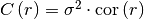
Given by: $C\left(r\right)= \sigma^2\cdot\mathrm{cor}\left(r\right)$

Where $\mathrm{cor}(r)$ is the correlation function.

default_arg_bounds()[source]¶

Provide default boundaries for arguments.

Given as a dictionary.

default_opt_arg()[source]¶

Defaults for the optional arguments.

{"hurst": 0.5, "len_low": 0.0}

Returns:	Defaults for optional arguments
Return type:	`dict`

default_opt_arg_bounds()[source]¶

Defaults for boundaries of the optional arguments.

{"hurst": [0, 1, "oo"], "len_low": [0, 1000, "cc"]}

Returns:	Boundaries for optional arguments
Return type:	`dict`

var_factor()[source]¶

Factor for C (Power-Law factor) to result in variance.

This is used to result in the right variance, which is depending on the hurst coefficient and the length-scale extents

$\frac{\ell_{\mathrm{up}}^{2H} - \ell_{\mathrm{low}}^{2H}}{2H}$

Returns:	factor
Return type:	`float`

variogram(r)¶

Isotropic variogram of the model.

Given by: $\gamma\left(r\right)= \sigma^2\cdot\left(1-\mathrm{cor}\left(r\right)\right)+n$

Where $\mathrm{cor}(r)$ is the correlation function.

len_up¶

Upper length scale truncation of the model.

len_up = len_low + len_scale

Type:	`float`

class gstools.covmodel.tpl_models.TPLExponential(dim=3, var=1.0, len_scale=1.0, nugget=0.0, anis=1.0, angles=0.0, integral_scale=None, var_raw=None, hankel_kw=None, **opt_arg)[source]¶

Bases: gstools.covmodel.base.CovModel

Truncated-Power-Law with Exponential modes.

Notes

The truncated power law is given by a superposition of scale-dependent variograms:

$\gamma_{\ell_{\mathrm{low}},\ell_{\mathrm{up}}}(r) = \intop_{\ell_{\mathrm{low}}}^{\ell_{\mathrm{up}}} \gamma(r,\lambda) \frac{\rm d \lambda}{\lambda}$

with Exponential modes on each scale:

$\gamma(r,\lambda) &= \sigma^2(\lambda)\cdot\left(1- \exp\left[- \frac{r}{\lambda}\right] \right)\\ \sigma^2(\lambda) &= C\cdot\lambda^{2H}$

This results in:

$\gamma_{\ell_{\mathrm{low}},\ell_{\mathrm{up}}}(r) &= \sigma^2_{\ell_{\mathrm{low}},\ell_{\mathrm{up}}}\cdot\left(1- 2H \cdot \frac{\ell_{\mathrm{up}}^{2H} \cdot E_{1+2H}\left[\frac{r}{\ell_{\mathrm{up}}}\right] - \ell_{\mathrm{low}}^{2H} \cdot E_{1+2H}\left[\frac{r}{\ell_{\mathrm{low}}}\right]} {\ell_{\mathrm{up}}^{2H}-\ell_{\mathrm{low}}^{2H}} \right) \\ \sigma^2_{\ell_{\mathrm{low}},\ell_{\mathrm{up}}} &= \frac{C\cdot\left(\ell_{\mathrm{up}}^{2H} -\ell_{\mathrm{low}}^{2H}\right)}{2H}$

The “length scale” of this model is equivalent by the integration range:

$\ell = \ell_{\mathrm{up}} -\ell_{\mathrm{low}}$

If you want to define an upper scale truncation, you should set len_low and len_scale accordingly.

The following Parameters occure:

$C>0$ : The scaling factor from the Power-Law. This parameter will be calculated internally by the given variance. You can access C directly by model.var_raw

$0<H<\frac{1}{2}$ : The hurst coefficient (model.hurst)

$\ell_{\mathrm{low}}\geq 0$ : The lower length scale truncation of the model (model.len_low)

$\ell_{\mathrm{up}}\geq 0$ : The upper length scale truncation of the model (model.len_up)

This will be calculated internally by:

len_up = len_low + len_scale

That means, that the len_scale in this model actually represents the integration range for the truncated power law.

$E_s(x)$ is the exponential integral.

Other Parameters:
	opt_arg – The following parameters are covered by these keyword arguments hurst (`float`, optional) – Hurst coefficient of the power law. Standard range: `(0, 1)`. Default: `0.5` len_low** (`float`, optional) – The lower length scale truncation of the model. Standard range: `[0, 1000]`. Default: `0.0` .
Parameters:	dim (`int`, optional) – dimension of the model. Default: `3` var (`float`, optional) – variance of the model (the nugget is not included in “this” variance) Default: `1.0` len_scale (`float` or `list`, optional) – length scale of the model. If a single value is given, the same length-scale will be used for every direction. If multiple values (for main and transversal directions) are given, anis will be recalculated accordingly. Default: `1.0` nugget (`float`, optional) – nugget of the model. Default: `0.0` anis (`float` or `list`, optional) – anisotropy ratios in the transversal directions [y, z]. Default: `1.0` angles (`float` or `list`, optional) – angles of rotation: in 2D: given as rotation around z-axis in 3D: given by yaw, pitch, and roll (known as Tait–Bryan angles) Default: `0.0` integral_scale (`float` or `list` or `None`, optional) – If given, `len_scale` will be ignored and recalculated, so that the integral scale of the model matches the given one. Default: `None` var_raw (`float` or `None`, optional) – raw variance of the model which will be multiplied with `CovModel.var_factor` to result in the actual variance. If given, `var` will be ignored. (This is just for models that override `CovModel.var_factor`) Default: `None` hankel_kw (`dict` or `None`, optional) – Modify the init-arguments of `hankel.SymmetricFourierTransform` used for the spectrum calculation. Use with caution (Better: Don’t!). `None` is equivalent to `{"a": -1, "b": 1, "N": 1000, "h": 0.001}`.
Attributes:	`angles` `numpy.ndarray`: Rotation angles (in rad) of the model. `anis` `numpy.ndarray`: The anisotropy factors of the model. `arg` `list` of `str`: Names of all arguments. `arg_bounds` `dict`: Bounds for all parameters. `dim` `int`: The dimension of the model. `dist_func` `tuple` of `callable`: pdf, cdf and ppf. `do_rotation` `bool`: State if a rotation is performed. `hankel_kw` `dict`: `hankel.SymmetricFourierTransform` kwargs. `has_cdf` `bool`: State if a cdf is defined by the user. `has_ppf` `bool`: State if a ppf is defined by the user. `integral_scale` `float`: The main integral scale of the model. `integral_scale_vec` `numpy.ndarray`: The integral scales in each direction. `len_scale` `float`: The main length scale of the model. `len_scale_bounds` `list`: Bounds for the lenght scale. `len_scale_vec` `numpy.ndarray`: The length scales in each direction. `len_up` `float`: Upper length scale truncation of the model. `name` `str`: The name of the CovModel class. `nugget` `float`: The nugget of the model. `nugget_bounds` `list`: Bounds for the nugget. `opt_arg` `list` of `str`: Names of the optional arguments. `opt_arg_bounds` `dict`: Bounds for the optional arguments. `pykrige_angle` 2D rotation angle for pykrige. `pykrige_angle_x` 3D rotation angle around x for pykrige. `pykrige_angle_y` 3D rotation angle around y for pykrige. `pykrige_angle_z` 3D rotation angle around z for pykrige. `pykrige_anis` 2D anisotropy ratio for pykrige. `pykrige_anis_y` 3D anisotropy ratio in y direction for pykrige. `pykrige_anis_z` 3D anisotropy ratio in z direction for pykrige. `pykrige_kwargs` Keyword arguments for pykrige routines. `sill` `float`: The sill of the variogram. `var` `float`: The variance of the model. `var_bounds` `list`: Bounds for the variance. `var_raw` `float`: The raw variance of the model without factor.

Methods

`calc_integral_scale`()	Calculate the integral scale of the isotrope model.
`check_arg_bounds`()	Check arguments to be within the given bounds.
`check_opt_arg`()	Run checks for the optional arguments.
`cor_spatial`(pos)	Spatial correlation respecting anisotropy and rotation.
`correlation`(r)	Truncated-Power-Law with Exponential modes - correlation function.
`cov_nugget`(r)	Covariance of the model respecting the nugget at r=0.
`cov_spatial`(pos)	Spatial covariance respecting anisotropy and rotation.
`covariance`(r)	Covariance of the model.
`default_arg_bounds`()	Provide default boundaries for arguments.
`default_opt_arg`()	Defaults for the optional arguments.
`default_opt_arg_bounds`()	Defaults for boundaries of the optional arguments.
`fit_variogram`(x_data, y_data[, maxfev])	Fiting the isotropic variogram-model to given data.
`fix_dim`()	Set a fix dimension for the model.
`ln_spectral_rad_pdf`(r)	Log radial spectral density of the model.
`percentile_scale`([per])	Calculate the percentile scale of the isotrope model.
`plot`([func])	Plot a function of a the CovModel.
`pykrige_vario`([args, r])	Isotropic variogram of the model for pykrige.
`set_arg_bounds`(**kwargs)	Set bounds for the parameters of the model.
`spectral_density`(k)	Spectral density of the covariance model.
`spectral_rad_pdf`(r)	Radial spectral density of the model.
`spectrum`(k)	Spectrum of the covariance model.
`var_factor`()	Factor for C (Power-Law factor) to result in variance.
`vario_nugget`(r)	Isotropic variogram of the model respecting the nugget at r=0.
`vario_spatial`(pos)	Spatial variogram respecting anisotropy and rotation.
`variogram`(r)	Isotropic variogram of the model.

correlation(r)[source]¶

Truncated-Power-Law with Exponential modes - correlation function.

If len_low=0 we have a simple representation:

$\mathrm{cor}(r) = H \cdot E_{1+H} \left[ \frac{r}{\ell} \right]$

The general case:

$\mathrm{cor}(r) = 2H \cdot \frac{\ell_{\mathrm{up}}^{2H} \cdot E_{1+2H}\left[\frac{r}{\ell_{\mathrm{up}}}\right] - \ell_{\mathrm{low}}^{2H} \cdot E_{1+2H}\left[\frac{r}{\ell_{\mathrm{low}}}\right]} {\ell_{\mathrm{up}}^{2H}-\ell_{\mathrm{low}}^{2H}}$

covariance(r)¶

Covariance of the model.

Given by: $C\left(r\right)= \sigma^2\cdot\mathrm{cor}\left(r\right)$

Where $\mathrm{cor}(r)$ is the correlation function.

default_arg_bounds()[source]¶

Provide default boundaries for arguments.

Given as a dictionary.

default_opt_arg()[source]¶

Defaults for the optional arguments.

{"hurst": 0.25, "len_low": 0.0}

Returns:	Defaults for optional arguments
Return type:	`dict`

default_opt_arg_bounds()[source]¶

Defaults for boundaries of the optional arguments.

{"hurst": [0, 1, "oo"], "len_low": [0, 1000, "cc"]}

Returns:	Boundaries for optional arguments
Return type:	`dict`

var_factor()[source]¶

Factor for C (Power-Law factor) to result in variance.

This is used to result in the right variance, which is depending on the hurst coefficient and the length-scale extents

$\frac{\ell_{\mathrm{up}}^{2H} - \ell_{\mathrm{low}}^{2H}}{2H}$

Returns:	factor
Return type:	`float`

variogram(r)¶

Isotropic variogram of the model.

Given by: $\gamma\left(r\right)= \sigma^2\cdot\left(1-\mathrm{cor}\left(r\right)\right)+n$

Where $\mathrm{cor}(r)$ is the correlation function.

len_up¶

Upper length scale truncation of the model.

len_up = len_low + len_scale

Type:	`float`

class gstools.covmodel.tpl_models.TPLStable(dim=3, var=1.0, len_scale=1.0, nugget=0.0, anis=1.0, angles=0.0, integral_scale=None, var_raw=None, hankel_kw=None, **opt_arg)[source]¶

Bases: gstools.covmodel.base.CovModel

Truncated-Power-Law with Stable modes.

Notes

The truncated power law is given by a superposition of scale-dependent variograms:

$\gamma_{\ell_{\mathrm{low}},\ell_{\mathrm{up}}}(r) = \intop_{\ell_{\mathrm{low}}}^{\ell_{\mathrm{up}}} \gamma(r,\lambda) \frac{\rm d \lambda}{\lambda}$

with Stable modes on each scale:

$\gamma(r,\lambda) &= \sigma^2(\lambda)\cdot\left(1- \exp\left[- \left(\frac{r}{\lambda}\right)^{\alpha}\right] \right)\\ \sigma^2(\lambda) &= C\cdot\lambda^{2H}$

This results in:

$\gamma_{\ell_{\mathrm{low}},\ell_{\mathrm{up}}}(r) &= \sigma^2_{\ell_{\mathrm{low}},\ell_{\mathrm{up}}}\cdot\left(1- \frac{2H}{\alpha} \cdot \frac{\ell_{\mathrm{up}}^{2H} \cdot E_{1+\frac{2H}{\alpha}} \left[\left(\frac{r}{\ell_{\mathrm{up}}}\right)^{\alpha}\right] - \ell_{\mathrm{low}}^{2H} \cdot E_{1+\frac{2H}{\alpha}} \left[\left(\frac{r}{\ell_{\mathrm{low}}}\right)^{\alpha}\right]} {\ell_{\mathrm{up}}^{2H}-\ell_{\mathrm{low}}^{2H}} \right) \\ \sigma^2_{\ell_{\mathrm{low}},\ell_{\mathrm{up}}} &= \frac{C\cdot\left(\ell_{\mathrm{up}}^{2H} -\ell_{\mathrm{low}}^{2H}\right)}{2H}$

The “length scale” of this model is equivalent by the integration range:

$\ell = \ell_{\mathrm{up}} -\ell_{\mathrm{low}}$

If you want to define an upper scale truncation, you should set len_low and len_scale accordingly.

The following Parameters occure:

$0<\alpha\leq 2$ : The shape parameter of the Stable model.

$\alpha=1$ : Exponential modes

$\alpha=2$ : Gaussian modes

$C>0$ : The scaling factor from the Power-Law. This parameter will be calculated internally by the given variance. You can access C directly by model.var_raw

$0<H<\frac{\alpha}{2}$ : The hurst coefficient (model.hurst)

$\ell_{\mathrm{low}}\geq 0$ : The lower length scale truncation of the model (model.len_low)

$\ell_{\mathrm{up}}\geq 0$ : The upper length scale truncation of the model (model.len_up)

This will be calculated internally by:

len_up = len_low + len_scale

That means, that the len_scale in this model actually represents the integration range for the truncated power law.

$E_s(x)$ is the exponential integral.

Other Parameters:
	opt_arg – The following parameters are covered by these keyword arguments hurst (`float`, optional) – Hurst coefficient of the power law. Standard range: `(0, 1)`. Default: `0.5` alpha (`float`, optional) – Shape parameter of the stable model. Standard range: `(0, 2]`. Default: `1.5` len_low** (`float`, optional) – The lower length scale truncation of the model. Standard range: `[0, 1000]`. Default: `0.0` .
Parameters:	dim (`int`, optional) – dimension of the model. Default: `3` var (`float`, optional) – variance of the model (the nugget is not included in “this” variance) Default: `1.0` len_scale (`float` or `list`, optional) – length scale of the model. If a single value is given, the same length-scale will be used for every direction. If multiple values (for main and transversal directions) are given, anis will be recalculated accordingly. Default: `1.0` nugget (`float`, optional) – nugget of the model. Default: `0.0` anis (`float` or `list`, optional) – anisotropy ratios in the transversal directions [y, z]. Default: `1.0` angles (`float` or `list`, optional) – angles of rotation: in 2D: given as rotation around z-axis in 3D: given by yaw, pitch, and roll (known as Tait–Bryan angles) Default: `0.0` integral_scale (`float` or `list` or `None`, optional) – If given, `len_scale` will be ignored and recalculated, so that the integral scale of the model matches the given one. Default: `None` var_raw (`float` or `None`, optional) – raw variance of the model which will be multiplied with `CovModel.var_factor` to result in the actual variance. If given, `var` will be ignored. (This is just for models that override `CovModel.var_factor`) Default: `None` hankel_kw (`dict` or `None`, optional) – Modify the init-arguments of `hankel.SymmetricFourierTransform` used for the spectrum calculation. Use with caution (Better: Don’t!). `None` is equivalent to `{"a": -1, "b": 1, "N": 1000, "h": 0.001}`.
Attributes:	`angles` `numpy.ndarray`: Rotation angles (in rad) of the model. `anis` `numpy.ndarray`: The anisotropy factors of the model. `arg` `list` of `str`: Names of all arguments. `arg_bounds` `dict`: Bounds for all parameters. `dim` `int`: The dimension of the model. `dist_func` `tuple` of `callable`: pdf, cdf and ppf. `do_rotation` `bool`: State if a rotation is performed. `hankel_kw` `dict`: `hankel.SymmetricFourierTransform` kwargs. `has_cdf` `bool`: State if a cdf is defined by the user. `has_ppf` `bool`: State if a ppf is defined by the user. `integral_scale` `float`: The main integral scale of the model. `integral_scale_vec` `numpy.ndarray`: The integral scales in each direction. `len_scale` `float`: The main length scale of the model. `len_scale_bounds` `list`: Bounds for the lenght scale. `len_scale_vec` `numpy.ndarray`: The length scales in each direction. `len_up` `float`: Upper length scale truncation of the model. `name` `str`: The name of the CovModel class. `nugget` `float`: The nugget of the model. `nugget_bounds` `list`: Bounds for the nugget. `opt_arg` `list` of `str`: Names of the optional arguments. `opt_arg_bounds` `dict`: Bounds for the optional arguments. `pykrige_angle` 2D rotation angle for pykrige. `pykrige_angle_x` 3D rotation angle around x for pykrige. `pykrige_angle_y` 3D rotation angle around y for pykrige. `pykrige_angle_z` 3D rotation angle around z for pykrige. `pykrige_anis` 2D anisotropy ratio for pykrige. `pykrige_anis_y` 3D anisotropy ratio in y direction for pykrige. `pykrige_anis_z` 3D anisotropy ratio in z direction for pykrige. `pykrige_kwargs` Keyword arguments for pykrige routines. `sill` `float`: The sill of the variogram. `var` `float`: The variance of the model. `var_bounds` `list`: Bounds for the variance. `var_raw` `float`: The raw variance of the model without factor.

Methods

`calc_integral_scale`()	Calculate the integral scale of the isotrope model.
`check_arg_bounds`()	Check arguments to be within the given bounds.
`check_opt_arg`()	Check the optional arguments.
`cor_spatial`(pos)	Spatial correlation respecting anisotropy and rotation.
`correlation`(r)	Truncated-Power-Law with Stable modes - correlation function.
`cov_nugget`(r)	Covariance of the model respecting the nugget at r=0.
`cov_spatial`(pos)	Spatial covariance respecting anisotropy and rotation.
`covariance`(r)	Covariance of the model.
`default_arg_bounds`()	Provide default boundaries for arguments.
`default_opt_arg`()	Defaults for the optional arguments.
`default_opt_arg_bounds`()	Defaults for boundaries of the optional arguments.
`fit_variogram`(x_data, y_data[, maxfev])	Fiting the isotropic variogram-model to given data.
`fix_dim`()	Set a fix dimension for the model.
`ln_spectral_rad_pdf`(r)	Log radial spectral density of the model.
`percentile_scale`([per])	Calculate the percentile scale of the isotrope model.
`plot`([func])	Plot a function of a the CovModel.
`pykrige_vario`([args, r])	Isotropic variogram of the model for pykrige.
`set_arg_bounds`(**kwargs)	Set bounds for the parameters of the model.
`spectral_density`(k)	Spectral density of the covariance model.
`spectral_rad_pdf`(r)	Radial spectral density of the model.
`spectrum`(k)	Spectrum of the covariance model.
`var_factor`()	Factor for C (Power-Law factor) to result in variance.
`vario_nugget`(r)	Isotropic variogram of the model respecting the nugget at r=0.
`vario_spatial`(pos)	Spatial variogram respecting anisotropy and rotation.
`variogram`(r)	Isotropic variogram of the model.

check_opt_arg()[source]¶

Check the optional arguments.

Warns:	alpha – If alpha is < 0.3, the model tends to a nugget model and gets numerically unstable.

correlation(r)[source]¶

Truncated-Power-Law with Stable modes - correlation function.

If len_low=0 we have a simple representation:

$\mathrm{cor}(r) = \frac{2H}{\alpha} \cdot E_{1+\frac{2H}{\alpha}} \left[ \left(\frac{r}{\ell}\right)^{\alpha} \right]$

The general case:

$\mathrm{cor}(r) = \frac{2H}{\alpha} \cdot \frac{\ell_{\mathrm{up}}^{2H} \cdot E_{1+\frac{2H}{\alpha}} \left[\left(\frac{r}{\ell_{\mathrm{up}}}\right)^{\alpha}\right] - \ell_{\mathrm{low}}^{2H} \cdot E_{1+\frac{2H}{\alpha}} \left[\left(\frac{r}{\ell_{\mathrm{low}}}\right)^{\alpha}\right]} {\ell_{\mathrm{up}}^{2H}-\ell_{\mathrm{low}}^{2H}}$

covariance(r)¶

Covariance of the model.

Given by: $C\left(r\right)= \sigma^2\cdot\mathrm{cor}\left(r\right)$

Where $\mathrm{cor}(r)$ is the correlation function.

default_arg_bounds()[source]¶

Provide default boundaries for arguments.

Given as a dictionary.

default_opt_arg()[source]¶

Defaults for the optional arguments.

{"hurst": 0.5, "alpha": 1.5, "len_low": 0.0}

Returns:	Defaults for optional arguments
Return type:	`dict`

default_opt_arg_bounds()[source]¶

Defaults for boundaries of the optional arguments.

{"hurst": [0, 1, "oo"], "alpha": [0, 2, "oc"], "len_low": [0, 1000, "cc"]}

Returns:	Boundaries for optional arguments
Return type:	`dict`

var_factor()[source]¶

Factor for C (Power-Law factor) to result in variance.

This is used to result in the right variance, which is depending on the hurst coefficient and the length-scale extents

$\frac{\ell_{\mathrm{up}}^{2H} - \ell_{\mathrm{low}}^{2H}}{2H}$

Returns:	factor
Return type:	`float`

variogram(r)¶

Isotropic variogram of the model.

Given by: $\gamma\left(r\right)= \sigma^2\cdot\left(1-\mathrm{cor}\left(r\right)\right)+n$

Where $\mathrm{cor}(r)$ is the correlation function.

len_up¶

Upper length scale truncation of the model.

len_up = len_low + len_scale

Type:	`float`