Tutorial 3: Variogram Estimation
Estimating the spatial correlations is an important part of geostatistics.
These spatial correlations can be expressed by the variogram, which can be
estimated with the subpackage gstools.variogram. The variograms can be
estimated on structured and unstructured grids.
Theoretical Background
The same (semi-)variogram as the Covariance Model is being used by this subpackage.
An Example with Actual Data
This example is going to be a bit more extensive and we are going to do some basic data preprocessing for the actual variogram estimation. But this example will be self-contained and all data gathering and processing will be done in this example script.
The complete script can be found in gstools/examples/08_variogram_estimation.py
This example will only work with Python 3.
The Data
We are going to analyse the Herten aquifer, which is situated in Southern Germany. Multiple outcrop faces where surveyed and interpolated to a 3D dataset. In these publications, you can find more information about the data:
Retrieving the Data
To begin with, we need to download and extract the data. Therefore, we are going to use some built-in Python libraries. For simplicity, many values and strings will be hardcoded.
import os
import urllib.request
import zipfile
import numpy as np
import matplotlib.pyplot as pt

def download_herten():
    # download the data, warning: its about 250MB
    print('Downloading Herten data')
    data_filename = 'data.zip'
    data_url = 'http://store.pangaea.de/Publications/Bayer_et_al_2015/Herten-analog.zip'
    urllib.request.urlretrieve(data_url, 'data.zip')

    # extract the data
    with zipfile.ZipFile(data_filename, 'r') as zf:
        zf.extract(os.path.join('Herten-analog', 'sim-big_1000x1000x140',
                                'sim.vtk'))
That was that. But we also need a script to convert the data into a format we can use. This script is also kindly provided by the authors. We can download this script in a very similar manner as the data:
def download_scripts():
    # download a script for file conversion
    print('Downloading scripts')
    tools_filename = 'scripts.zip'
    tool_url = 'http://store.pangaea.de/Publications/Bayer_et_al_2015/tools.zip'
    urllib.request.urlretrieve(tool_url, tools_filename)

    # only extract the script we need
    with zipfile.ZipFile(tools_filename, 'r') as zf:
        zf.extract(os.path.join('tools', 'vtk2gslib.py'))
These two functions can now be called:
download_herten()
download_scripts()
Preprocessing the Data
First of all, we have to convert the data with the script we just downloaded
# import the downloaded conversion script
from tools.vtk2gslib import vtk2numpy

# load the Herten aquifer with the downloaded vtk2numpy routine
print('Loading data')
herten, grid = vtk2numpy(os.path.join('Herten-analog', 'sim-big_1000x1000x140', 'sim.vtk'))
The data only contains facies, but from the supplementary data, we know the hydraulic conductivity values of each facies, which we will simply paste here and assign them to the correct facies
# conductivity values per fazies from the supplementary data
cond = np.array([2.50E-04, 2.30E-04, 6.10E-05, 2.60E-02, 1.30E-01,
                 9.50E-02, 4.30E-05, 6.00E-07, 2.30E-03, 1.40E-04,])

# asign the conductivities to the facies
herten_cond = cond[herten]
Next, we are going to calculate the transmissivity, by integrating over the vertical axis
# integrate over the vertical axis, calculate transmissivity
herten_log_trans = np.log(np.sum(herten_cond, axis=2) * grid['dz'])
The Herten data provides information about the grid, which was already used in the previous code block. From this information, we can create our own grid on which we can estimate the variogram. As a first step, we are going to estimate an isotropic variogram, meaning that we will take point pairs from all directions into account. An unstructured grid is a natural choice for this. Therefore, we are going to create an unstructured grid from the given, structured one. For this, we are going to write another small function
def create_unstructured_grid(x_s, y_s):
    x_u, y_u = np.meshgrid(x_s, y_s)
    len_unstruct = len(x_s) * len(y_s)
    x_u = np.reshape(x_u, len_unstruct)
    y_u = np.reshape(y_u, len_unstruct)
    return x_u, y_u

# create a structured grid on which the data is defined
x_s = np.arange(grid['ox'], grid['nx']*grid['dx'], grid['dx'])
y_s = np.arange(grid['oy'], grid['ny']*grid['dy'], grid['dy'])

# create an unstructured grid for the variogram estimation
x_u, y_u = create_unstructured_grid(x_s, y_s)
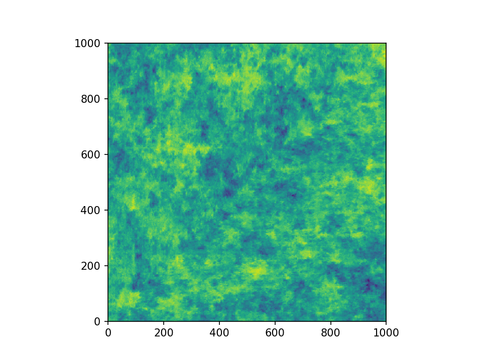
Let’s have a look at the transmissivity field of the Herten aquifer
pt.imshow(herten_log_trans.T, origin='lower', aspect='equal')
pt.show()
Estimating the Variogram
Finally, everything is ready for the variogram estimation. For the unstructured
method, we have to define the bins on which the variogram will be estimated.
Through expert knowledge (i.e. fiddling around), we assume that the main
features of the variogram will be below 10 metres distance. And because the
data has a high spatial resolution, the resolution of the bins can also be
high. The transmissivity data is still defined on a structured grid, but we can
simply flatten it with numpy.ndarray.flatten, in order to bring it into
the right shape. It might be more memory efficient to use
herten_log_trans.reshape(-1), but for better readability, we will stick to
numpy.ndarray.flatten. Taking all data points into account would take a
very long time (expert knowledge *wink*), thus we will only take 2000 datapoints into account, which are sampled randomly. In order to make the exact
results reproducible, we can also set a seed.
from gstools import vario_estimate_unstructured

bins = np.linspace(0, 10, 50)
print('Estimating unstructured variogram')
bin_center, gamma = vario_estimate_unstructured(
    (x_u, y_u),
    herten_log_trans.flatten(),
    bins,
    sampling_size=2000,
    sampling_seed=19920516,
    )
The estimated variogram is calculated on the centre of the given bins,
therefore, the bin_center array is also returned.
Fitting the Variogram
Now, we can see, if the estimated variogram can be modelled by a common
variogram model. Let’s try the Exponential model.
from gstools import Exponential

# fit an exponential model
fit_model = Exponential(dim=2)
fit_model.fit_variogram(bin_center, gamma, nugget=False)
Finally, we can visualise some results. For quickly plotting a covariance model, GSTools provides some helper functions.
from gstools.covmodel.plot import plot_variogram
pt.plot(bin_center, gamma)
plot_variogram(fit_model, x_max=bins[-1])
pt.show()
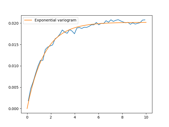
That looks like a pretty good fit! By printing the model, we can directly see the fitted parameters
print(fit_model)
which gives
Exponential(dim=2, var=0.020193095802479327, len_scale=1.4480057557321007, nugget=0.0, anis=[1.], angles=[0.])
With this data, we could start generating new ensembles of the Herten aquifer
with the SRF class.
Estimating the Variogram in Specific Directions
Estimating a variogram on a structured grid gives us the possibility to only consider values in a specific direction. This could be a first test, to see if the data is anisotropic. In order to speed up the calculations, we are going to only use every 10th datapoint and for a comparison with the isotropic variogram calculated earlier, we only need the first 21 array items.
x_s = x_s[::10][:21]
y_s = y_s[::10][:21]
herten_trans_log = herten_log_trans[::10,::10]
With this much smaller data set, we can immediately estimate the variogram in the x- and y-axis
from gstools import vario_estimate_structured
print('Estimating structured variograms')
gamma_x = vario_estimate_structured(herten_trans_log, direction='x')[:21]
gamma_y = vario_estimate_structured(herten_trans_log, direction='y')[:21]
With these two estimated variograms, we can start fitting Exponential
covariance models
fit_model_x = Exponential(dim=2)
fit_model_x.fit_variogram(x_s, gamma_x, nugget=False)
fit_model_y = Exponential(dim=2)
fit_model_y.fit_variogram(y_s, gamma_y, nugget=False)
Now, the isotropic variogram and the two variograms in x- and y-direction can be plotted together with their respective models, which will be plotted with dashed lines.
line, = pt.plot(bin_center, gamma, label='estimated variogram (isotropic)')
pt.plot(bin_center, fit_model.variogram(bin_center), color=line.get_color(),
        linestyle='--', label='exp. variogram (isotropic)')

line, = pt.plot(x_s, gamma_x, label='estimated variogram in x-dir')
pt.plot(x_s, fit_model_x.variogram(x_s), color=line.get_color(),
        linestyle='--', label='exp. variogram in x-dir')

line, = pt.plot(y_s, gamma_y, label='estimated variogram in y-dir')
pt.plot(y_s, fit_model_y.variogram(y_s),
    color=line.get_color(), linestyle='--', label='exp. variogram in y-dir')

pt.legend()
pt.show()
Giving
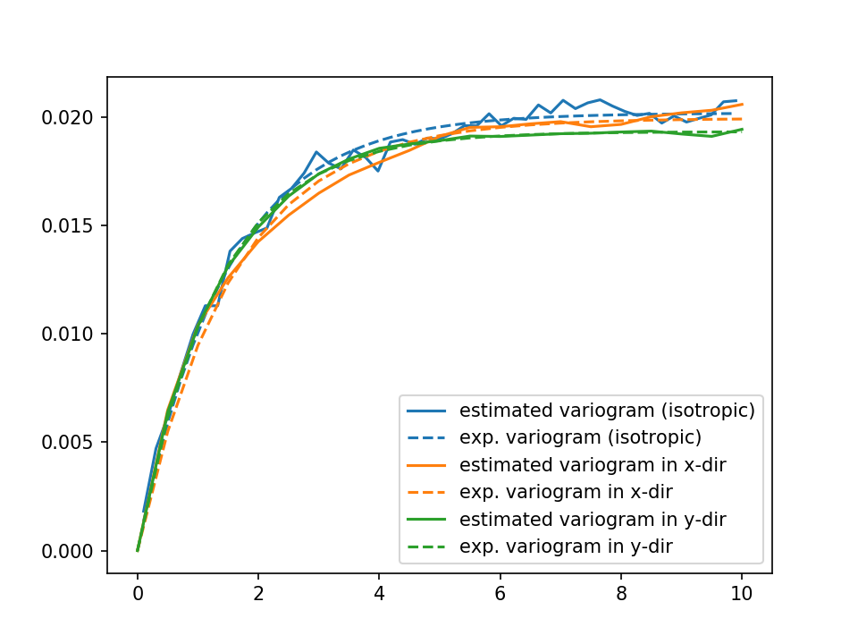
The plot might be a bit cluttered, but at least it is pretty obvious that the Herten aquifer has no apparent anisotropies in its spatial structure.
Creating a Spatial Random Field from the Herten Parameters
With all the hard work done, it’s straight forward now, to generate new Herten realisations
from gstools import SRF

srf = SRF(fit_model, seed=19770928)
new_herten = srf((x_s, y_s), mesh_type='structured')

pt.imshow(new_herten.T, origin='lower')
pt.show()
Yielding
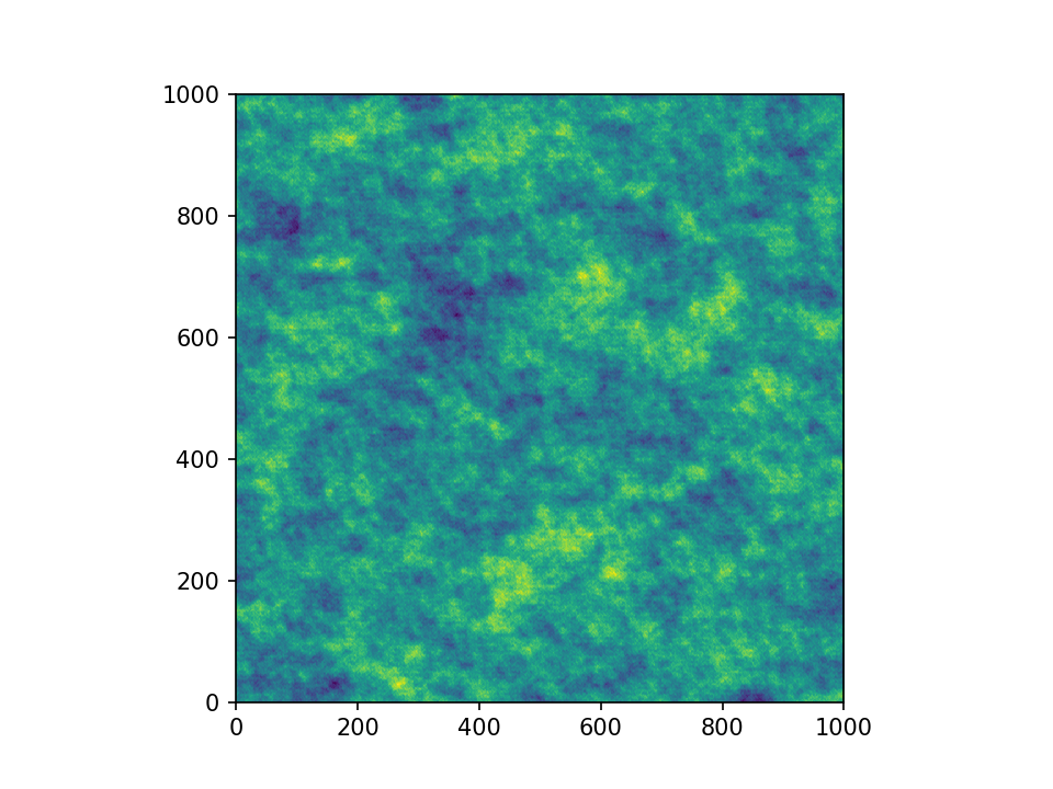
That’s pretty neat! Executing the code given on this site, will result in a lower resolution of the field, because we overwrote x_s and y_s for the directional variogram estimation. In the example script, this is not the case and you will get a high resolution field.
And Now for Some Cleanup
In case you want all the downloaded data and scripts to be deleted, use following commands
from shutil import rmtree
os.remove('data.zip')
os.remove('scripts.zip')
rmtree('Herten-analog')
rmtree('tools')
And in case you want to play around a little bit more with the data, you can
comment out the function calls download_herten() and
download_scripts(), after they where called at least once and also comment
out the cleanup. This way, the data will not be downloaded with every script
execution.