Tutorial 1: Random Field Generation¶

The main feature of GSTools is the spatial random field generator SRF, which can generate random fields following a given covariance model. The generator provides a lot of nice features, which will be explained in the following

Theoretical Background¶

GSTools generates spatial random fields with a given covariance model or semi-variogram. This is done by using the so-called randomization method. The spatial random field is represented by a stochastic Fourier integral and its discretised modes are evaluated at random frequencies.

GSTools supports arbitrary and non-isotropic covariance models.

A very Simple Example¶

We are going to start with a very simple example of a spatial random field with an isotropic Gaussian covariance model and following parameters:

variance $\sigma^2=1$
correlation length $\lambda=10$

First, we set things up and create the axes for the field. We are going to need the SRF class for the actual generation of the spatial random field. But SRF also needs a covariance model and we will simply take the Gaussian model.

from gstools import SRF, Gaussian

x = y = range(100)

Now we create the covariance model with the parameters $\sigma^2$ and $\lambda$ and hand it over to SRF. By specifying a seed, we make sure to create reproducible results:

model = Gaussian(dim=2, var=1, len_scale=10)
srf = SRF(model, seed=20170519)

With these simple steps, everything is ready to create our first random field. We will create the field on a structured grid (as you might have guessed from the x and y), which makes it easier to plot.

field = srf.structured([x, y])
srf.plot()

Yielding

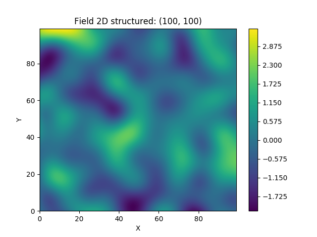
Wow, that was pretty easy!

The script can be found in gstools/examples/00_gaussian.py

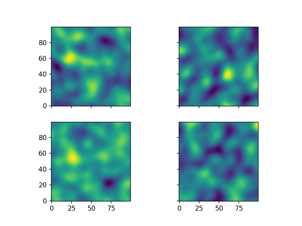
Creating an Ensemble of Fields¶

Creating an ensemble of random fields would also be a great idea. Let’s reuse most of the previous code.

import numpy as np
import matplotlib.pyplot as pt
from gstools import SRF, Gaussian

x = y = np.arange(100)

model = Gaussian(dim=2, var=1, len_scale=10)
srf = SRF(model)

This time, we did not provide a seed to SRF, as the seeds will used during the actual computation of the fields. We will create four ensemble members, for better visualisation and save them in a list and in a first step, we will be using the loop counter as the seeds.

ens_no = 4
field = []
for i in range(ens_no):
    field.append(srf.structured([x, y], seed=i))

Now let’s have a look at the results:

fig, ax = pt.subplots(2, 2, sharex=True, sharey=True)
ax = ax.flatten()
for i in range(ens_no):
    ax[i].imshow(field[i].T, origin='lower')
pt.show()

Yielding

The script can be found in gstools/examples/05_srf_ensemble.py

Using better Seeds¶

It is not always a good idea to use incrementing seeds. Therefore GSTools provides a seed generator MasterRNG. The loop, in which the fields are generated would then look like

from gstools.random import MasterRNG
seed = MasterRNG(20170519)
for i in range(ens_no):
    field.append(srf.structured([x, y], seed=seed()))

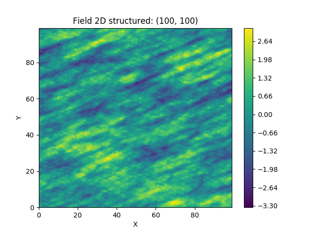
Creating Fancier Fields¶

Only using Gaussian covariance fields gets boring. Now we are going to create much rougher random fields by using an exponential covariance model and we are going to make them anisotropic.

The code is very similar to the previous examples, but with a different covariance model class Exponential. As model parameters we a using following

variance $\sigma^2=1$
correlation length $\lambda=(12, 3)^T$
rotation angle $\theta=\pi/8$

import numpy as np
from gstools import SRF, Exponential

x = y = np.arange(100)

model = Exponential(dim=2, var=1, len_scale=[12., 3.], angles=np.pi/8.)
srf = SRF(model, seed=20170519)

srf.structured([x, y])
srf.plot()

Yielding

The anisotropy ratio could also have been set with

model = Exponential(dim=2, var=1, len_scale=12., anis=3./12., angles=np.pi/8.)

Using an Unstructured Grid¶

For many applications, the random fields are needed on an unstructured grid. Normally, such a grid would be read in, but we can simply generate one and then create a random field at those coordinates.

import numpy as np
from gstools import SRF, Exponential
from gstools.random import MasterRNG

seed = MasterRNG(19970221)
rng = np.random.RandomState(seed())
x = rng.randint(0, 100, size=10000)
y = rng.randint(0, 100, size=10000)

model = Exponential(dim=2, var=1, len_scale=[12., 3.], angles=np.pi/8.)

srf = SRF(model, seed=20170519)
srf([x, y])
srf.plot()

Yielding

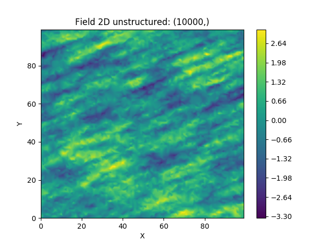
Comparing this image to the previous one, you can see that be using the same seed, the same field can be computed on different grids.

The script can be found in gstools/examples/06_unstr_srf_export.py

Exporting a Field¶

Using the field from previous example, it can simply be exported to the file field.vtu and viewed by e.g. paraview with following lines of code

srf.vtk_export("field")

Or it could visualized immediately in Python using PyVista:

mesh = srf.to_pyvista("field")
mesh.plot()

The script can be found in gstools/examples/04_export.py and in gstools/examples/06_unstr_srf_export.py

Merging two Fields¶

We can even generate the same field realisation on different grids. Let’s try to merge two unstructured rectangular fields. The first field will be generated exactly like in example Using an Unstructured Grid:

import numpy as np
import matplotlib.pyplot as pt
from gstools import SRF, Exponential
from gstools.random import MasterRNG

seed = MasterRNG(19970221)
rng = np.random.RandomState(seed())
x = rng.randint(0, 100, size=10000)
y = rng.randint(0, 100, size=10000)

model = Exponential(dim=2, var=1, len_scale=[12., 3.], angles=np.pi/8.)

srf = SRF(model, seed=20170519)

field = srf([x, y])

But now we extend the field on the right hand side by creating a new unstructured grid and calculating a field with the same parameters and the same seed on it:

# new grid
seed = MasterRNG(20011012)
rng = np.random.RandomState(seed())
x2 = rng.randint(99, 150, size=10000)
y2 = rng.randint(20, 80, size=10000)

field2 = srf((x2, y2))

pt.tricontourf(x, y, field.T)
pt.tricontourf(x2, y2, field2.T)
pt.axes().set_aspect('equal')
pt.show()

Yielding

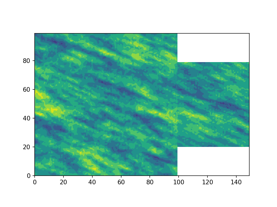
The slight mismatch where the two fields were merged is merely due to interpolation problems of the plotting routine. You can convince yourself be increasing the resolution of the grids by a factor of 10.

Of course, this merging could also have been done by appending the grid point (x2, y2) to the original grid (x, y) before generating the field. But one application scenario would be to generate hugh fields, which would not fit into memory anymore.

The script can be found in gstools/examples/07_srf_merge.py