Tutorial 2: The Covariance Model
One of the core-features of GSTools is the powerful CovModel
class, which allows you to easily define arbitrary covariance models by
yourself. The resulting models provide a bunch of nice features to explore the
covariance models.
Theoretical Backgound
A covariance model is used to characterize the
semi-variogram,
denoted by  , of a spatial random field.
In GSTools, we use the following form for an isotropic and stationary field:
, of a spatial random field.
In GSTools, we use the following form for an isotropic and stationary field:

- Where:
 is the so called
correlation
function depending on the distance
is the so called
correlation
function depending on the distance 
 is the variance
 is the nugget (subscale variance)
Note
We are not limited to isotropic models. We support anisotropy ratios for length scales in orthogonal transversal directions like:
 (main direction)
 (1. transversal direction)
 (2. transversal direction)
These main directions can also be rotated, but we will come to that later.
Example
Let us start with a short example of a self defined model (Of course, we
provide a lot of predefined models [See: gstools.covmodel],
but they all work the same way).
Therefore we reimplement the Gaussian covariance model by defining just the
correlation function:
from gstools import CovModel
import numpy as np
# use CovModel as the base-class
class Gau(CovModel):
    def correlation(self, r):
        return np.exp(-(r/self.len_scale)**2)
Now we can instantiate this model:
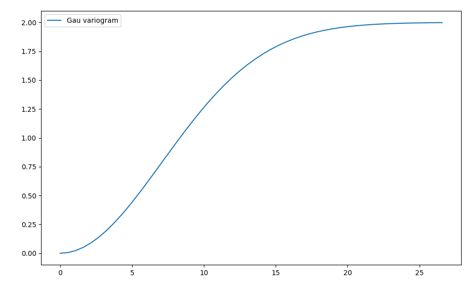
model = Gau(dim=2, var=2., len_scale=10)
To have a look at the variogram, let’s plot it:
from gstools.covmodel.plot import plot_variogram
plot_variogram(model)
Which gives:
Parameters
We already used some parameters, which every covariance models has. The basic ones are:
- dim : dimension of the model
- var : variance of the model (on top of the subscale variance)
- len_scale : length scale of the model
- nugget : nugget (subscale variance) of the model
These are the common parameters used to characterize a covariance model and are therefore used by every model in GSTools. You can also access and reset them:
print(model.dim, model.var, model.len_scale, model.nugget, model.sill)
model.dim = 3
model.var = 1
model.len_scale = 15
model.nugget = 0.1
print(model.dim, model.var, model.len_scale, model.nugget, model.sill)
Which gives:
2 2.0 10 0.0 2.0
3 1.0 15 0.1 1.1
Note
- The sill of the variogram is calculated by
sill = variance + nuggetSo we treat the variance as everything above the nugget, which is sometimes called partial sill. - A covariance model can also have additional parameters.
Anisotropy
The internally used (semi-) variogram represents the isotropic case for the model. Nevertheless, you can provide anisotropy ratios by:
model = Gau(dim=3, var=2., len_scale=10, anis=0.5)
print(model.anis)
print(model.len_scale_vec)
Which gives:
[0.5 1. ]
[10.  5. 10.]
As you can see, we defined just one anisotropy-ratio and the second transversal
direction was filled up with 1. and you can get the length-scales in each
direction by the attribute len_scale_vec. For full control you can set
a list of anistropy ratios: anis=[0.5, 0.4].
Alternatively you can provide a list of length-scales:
model = Gau(dim=3, var=2., len_scale=[10, 5, 4])
print(model.anis)
print(model.len_scale)
print(model.len_scale_vec)
Which gives:
[0.5 0.4]
10
[10.  5.  4.]
Rotation Angles
The main directions of the field don’t have to coincide with the spatial
directions , and . Therefore you can provide
rotation angles for the model:
model = Gau(dim=3, var=2., len_scale=10, angles=2.5)
print(model.angles)
Which gives:
[2.5 0. 0. ]
Again, the angles were filled up with 0. to match the dimension and you
could also provide a list of angles. The number of angles depends on the
given dimension:
- in 1D: no rotation performable
- in 2D: given as rotation around z-axis
- in 3D: given by yaw, pitch, and roll (known as Tait–Bryan angles)
Methods
The covariance model class CovModel of GSTools provides a set of handy
methods.
Basics
One of the following functions defines the main characterization of the variogram:
variogram: The variogram of the model given bycovariance: The (auto-)covariance of the model given by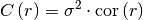
correlation: The (auto-)correlation (or normalized covariance) of the model given by
As you can see, it is the easiest way to define a covariance model by giving a
correlation function as demonstrated by the above model Gau.
If one of the above functions is given, the others will be determined:
model = Gau(dim=3, var=2., len_scale=10, nugget=0.5)
print(model.variogram(10.))
print(model.covariance(10.))
print(model.correlation(10.))
Which gives:
1.7642411176571153
0.6321205588285577
0.7357588823428847
0.36787944117144233
Spectral methods
The spectrum of a covariance model is given by:
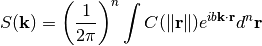
Since the covariance function  is radially symmetric, we can
calculate this by the
hankel-transformation:
is radially symmetric, we can
calculate this by the
hankel-transformation:
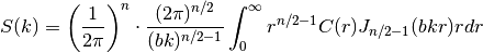
Where  .
.
Depending on the spectrum, the spectral-density is defined by:

You can access these methods by:
model = Gau(dim=3, var=2., len_scale=10)
print(model.spectrum(0.1))
print(model.spectral_density(0.1))
Which gives:
34.96564773852395
17.482823869261974
Note
The spectral-density is given by the radius of the input phase. But it is
not a probability density function for the radius of the phase.
To obtain the pdf for the phase-radius, you can use the methods
spectral_rad_pdf or ln_spectral_rad_pdf for the logarithm.
The user can also provide a cdf (cumulative distribution function) by
defining a method called spectral_rad_cdf and/or a ppf (percent-point function)
by spectral_rad_ppf.
Different scales
Besides the length-scale, there are many other ways of characterizing a certain scale of a covariance model. We provide two common scales with the covariance model.
Integral scale
The integral scale of a covariance model is calculated by:
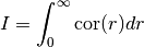
You can access it by:
model = Gau(dim=3, var=2., len_scale=10)
print(model.integral_scale)
print(model.integral_scale_vec)
Which gives:
8.862269254527579
[8.86226925 8.86226925 8.86226925]
You can also specify integral length scales like the ordinary length scale, and len_scale/anis will be recalculated:
model = Gau(dim=3, var=2., integral_scale=[10, 4, 2])
print(model.anis)
print(model.len_scale)
print(model.len_scale_vec)
print(model.integral_scale)
print(model.integral_scale_vec)
Which gives:
[0.4 0.2]
11.283791670955127
[11.28379167  4.51351667  2.25675833]
10.000000000000002
[10.  4.  2.]
Percentile scale
Another scale characterizing the covariance model, is the percentile scale. It is the distance, where the normalized variogram reaches a certain percentage of its sill.
model = Gau(dim=3, var=2., len_scale=10)
print(model.percentile_scale(0.9))
Which gives:
15.174271293851463
Note
The nugget is neglected by this percentile_scale.
Additional Parameters
Let’s pimp our self-defined model Gau by setting the exponent as an additional
parameter:
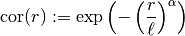
This leads to the so called stable covariance model and we can define it by
class Stab(CovModel):
    def default_opt_arg(self):
        return {"alpha": 1.5}
    def correlation(self, r):
        return np.exp(-(r/self.len_scale)**self.alpha)
As you can see, we override the method CovModel.default_opt_arg to provide
a standard value for the optional argument alpha and we can access it
in the correlation function by self.alpha
Now we can instantiate this model:
model1 = Stab(dim=2, var=2., len_scale=10)
model2 = Stab(dim=2, var=2., len_scale=10, alpha=0.5)
print(model1)
print(model2)
Which gives:
Stab(dim=2, var=2.0, len_scale=10, nugget=0.0, anis=[1.], angles=[0.], alpha=1.5)
Stab(dim=2, var=2.0, len_scale=10, nugget=0.0, anis=[1.], angles=[0.], alpha=0.5)
Note
You don’t have to overrid the CovModel.default_opt_arg, but you will
get a ValueError if you don’t set it on creation.
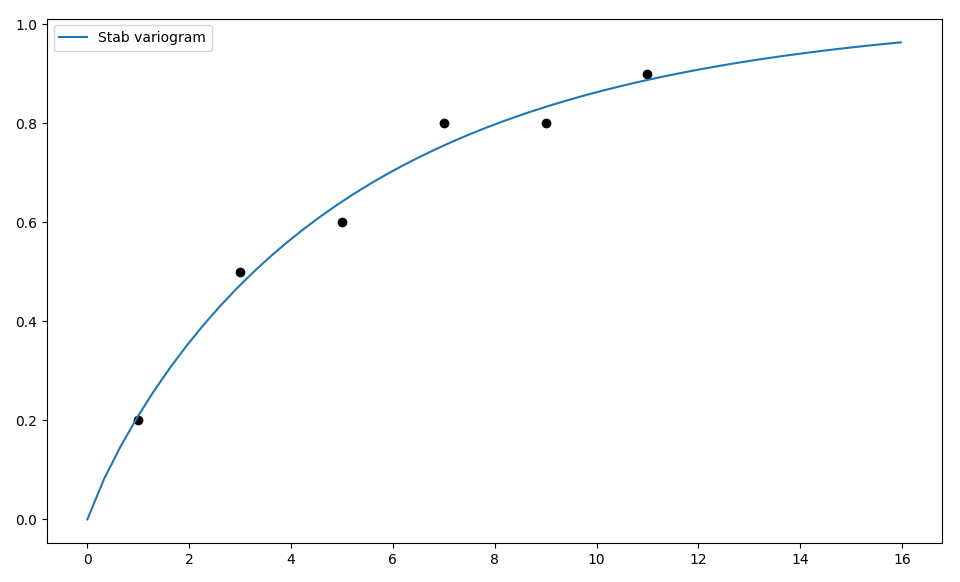
Fitting variogram data
The model class comes with a routine to fit the model-parameters to given variogram data. Have a look at the following:
# data
x = [1.0, 3.0, 5.0, 7.0, 9.0, 11.0]
y = [0.2, 0.5, 0.6, 0.8, 0.8, 0.9]
# fitting model
model = Stab(dim=2)
# we have to provide boundaries for the parameters
model.set_arg_bounds(alpha=[0, 3])
# fit the model to given data, deselect nugget
results, pcov = model.fit_variogram(x, y, nugget=False)
print(results)
# show the fitting
from matplotlib import pyplot as plt
from gstools.covmodel.plot import plot_variogram
plt.scatter(x, y, color="k")
plot_variogram(model)
plt.show()
Which gives:
{'var': 1.024575782651677,
 'len_scale': 5.081620691462197,
 'nugget': 0.0,
 'alpha': 0.906705123369987}
As you can see, we have to provide boundaries for the parameters. As a default, the following bounds are set:
- additional parameters:
[-np.inf, np.inf] - variance:
[0.0, np.inf] - len_scale:
[0.0, np.inf] - nugget:
[0.0, np.inf]
Also, you can deselect parameters from fitting, so their predefined values
will be kept. In our case, we fixed a nugget of 0.0, which was set
by default. You can deselect any standard or optional argument of the covariance model.
The second return value pcov is the estimated covariance of popt from
the used scipy routine scipy.optimize.curve_fit.
You can use the following methods to manipulate the used bounds:
CovModel.default_opt_arg_bounds() |
Provide default boundaries for optional arguments. |
CovModel.default_arg_bounds() |
Provide default boundaries for arguments. |
CovModel.set_arg_bounds(**kwargs) |
Set bounds for the parameters of the model. |
CovModel.check_arg_bounds() |
Check arguments to be within the given bounds. |
You can override the CovModel.default_opt_arg_bounds to provide standard
bounds for your additional parameters.
To access the bounds you can use:
CovModel.var_bounds |
Bounds for the variance. |
CovModel.len_scale_bounds |
Bounds for the lenght scale. |
CovModel.nugget_bounds |
Bounds for the nugget. |
CovModel.opt_arg_bounds |
Bounds for the optional arguments. |
CovModel.arg_bounds |
Bounds for all parameters. |
Provided Covariance Models
The following standard covariance models are provided by GSTools
Gaussian([dim, var, len_scale, nugget, …]) |
The Gaussian covariance model. |
Exponential([dim, var, len_scale, nugget, …]) |
The Exponential covariance model. |
Matern([dim, var, len_scale, nugget, anis, …]) |
The Matérn covariance model. |
Stable([dim, var, len_scale, nugget, anis, …]) |
The stable covariance model. |
Rational([dim, var, len_scale, nugget, …]) |
The rational quadratic covariance model. |
Linear([dim, var, len_scale, nugget, anis, …]) |
The bounded linear covariance model. |
Circular([dim, var, len_scale, nugget, …]) |
The circular covariance model. |
Spherical([dim, var, len_scale, nugget, …]) |
The Spherical covariance model. |
Intersection([dim, var, len_scale, nugget, …]) |
The Intersection covariance model. |
As a special feature, we also provide truncated power law (TPL) covariance models
TPLGaussian([dim, var, len_scale, nugget, …]) |
Truncated-Power-Law with Gaussian modes. |
TPLExponential([dim, var, len_scale, …]) |
Truncated-Power-Law with Exponential modes. |
TPLStable([dim, var, len_scale, nugget, …]) |
Truncated-Power-Law with Stable modes. |