Tutorial 5: Kriging
The subpackage gstools.krige provides routines for Gaussian process regression, also known as kriging.
Kriging is a method of data interpolation based on predefined covariance models.
We provide two kinds of kriging routines:
- Simple: The data is interpolated with a given mean value for the kriging field.
- Ordinary: The mean of the resulting field is unkown and estimated during interpolation.
Theoretical Background
The aim of kriging is to derive the value of a field at some point  ,
when there are fixed observed values
,
when there are fixed observed values  at given points
  .
.
The resluting value  at is calculated as a weighted mean:
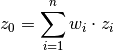
The weights  depent on the given covariance model and the location of the target point.
The different kriging approaches provide different ways of calculating  .
.
Implementation
The routines for kriging are almost identical to the routines for spatial random fields. First you define a covariance model, as described in the SRF tutorial, then you initialize the kriging class with this model:
from gstools import Gaussian, krige
# condtions
cond_pos = ...
cond_val = ...
model = Gaussian(dim=1, var=0.5, len_scale=2)
krig = krige.Simple(model, mean=1, cond_pos=cond_pos, cond_val=cond_val)
The resulting field instance krig has the same methods as the SRF class.
You can call it to evaluate the kriged field at different points,
you can plot the latest field or you can export the field and so on.
Have a look at the documentation of Simple and Ordinary.
Simple Kriging
Simple kriging assumes a known mean of the data. For simplicity we assume a mean of 0, which can be achieved by subtracting the mean from the observed values and subsequently adding it to the resulting data.
The resulting equation system for is given by:
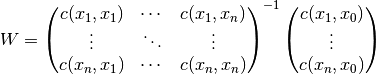
Thereby  is the covariance of the given observations.
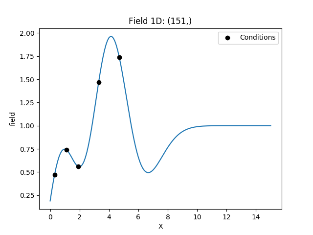
Example
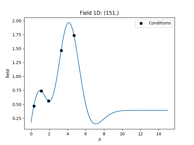
Here we use simple kriging in 1D (for plotting reasons) with 5 given observations/conditions. The mean of the field has to be given beforehand.
import numpy as np
from gstools import Gaussian, krige
# condtions
cond_pos = [0.3, 1.9, 1.1, 3.3, 4.7]
cond_val = [0.47, 0.56, 0.74, 1.47, 1.74]
# resulting grid
gridx = np.linspace(0.0, 15.0, 151)
# spatial random field class
model = Gaussian(dim=1, var=0.5, len_scale=2)
krig = krige.Simple(model, mean=1, cond_pos=cond_pos, cond_val=cond_val)
krig(gridx)
ax = krig.plot()
ax.scatter(cond_pos, cond_val, color="k", zorder=10, label="Conditions")
ax.legend()
Ordinary Kriging
Ordinary kriging will estimate an appropriate mean of the field, based on the given observations/conditions and the covariance model used.
The resulting system of equations for is given by:
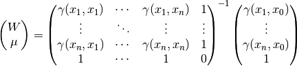
Thereby  is the semi-variogram of the given observations
and
is the semi-variogram of the given observations
and  is a Lagrange multiplier to minimize the kriging error and estimate the mean.
Example
Here we use ordinary kriging in 1D (for plotting reasons) with 5 given observations/conditions.
The estimated mean can be accessed by krig.mean.
import numpy as np
from gstools import Gaussian, krige
# condtions
cond_pos = [0.3, 1.9, 1.1, 3.3, 4.7]
cond_val = [0.47, 0.56, 0.74, 1.47, 1.74]
# resulting grid
gridx = np.linspace(0.0, 15.0, 151)
# spatial random field class
model = Gaussian(dim=1, var=0.5, len_scale=2)
krig = krige.Ordinary(model, cond_pos=cond_pos, cond_val=cond_val)
krig(gridx)
ax = krig.plot()
ax.scatter(cond_pos, cond_val, color="k", zorder=10, label="Conditions")
ax.legend()
Interface to PyKrige
To use fancier methods like universal kriging, we provide an interface to PyKrige.
You can pass a GSTools Covariance Model to the PyKrige routines as variogram_model.
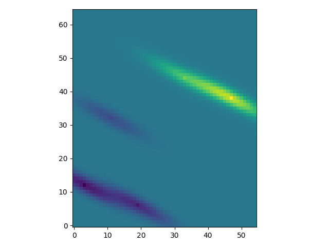
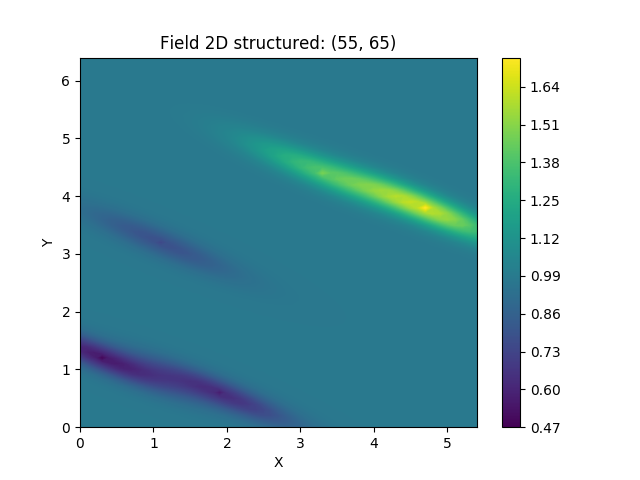
To demonstrate the general workflow, we compare the ordinary kriging of PyKrige with GSTools in 2D:
import numpy as np
from gstools import Gaussian, krige
from pykrige.ok import OrdinaryKriging
from matplotlib import pyplot as plt

# conditioning data
data = np.array([[0.3, 1.2, 0.47],
                 [1.9, 0.6, 0.56],
                 [1.1, 3.2, 0.74],
                 [3.3, 4.4, 1.47],
                 [4.7, 3.8, 1.74]])
# grid definition for output field
gridx = np.arange(0.0, 5.5, 0.1)
gridy = np.arange(0.0, 6.5, 0.1)
# a GSTools based covariance model
cov_model = Gaussian(dim=2, len_scale=1, anis=.2, angles=-.5, var=.5, nugget=.1)
# ordinary kriging with pykrige
OK1 = OrdinaryKriging(data[:, 0], data[:, 1], data[:, 2], cov_model)
z1, ss1 = OK1.execute('grid', gridx, gridy)
plt.imshow(z1, origin="lower")
plt.show()
# ordinary kriging with gstools for comparison
OK2 = krige.Ordinary(cov_model, [data[:, 0], data[:, 1]], data[:, 2])
OK2.structured([gridx, gridy])
OK2.plot()