Tutorial 4: Random Vector Field Generation¶

In 1970, Kraichnan was the first to suggest a randomization method. For studying the diffusion of single particles in a random incompressible velocity field, he came up with a randomization method which includes a projector which ensures the incompressibility of the vector field.

Theoretical Background¶

Without loss of generality we assume that the mean velocity $\bar{U}$ is oriented towards the direction of the first basis vector $\mathbf{e}_1$ . Our goal is now to generate random fluctuations with a given covariance model around this mean velocity. And at the same time, making sure that the velocity field remains incompressible or in other words, ensure $\nabla \cdot \mathbf U = 0$ . This can be done by using the randomization method we already know, but adding a projector to every mode being summed:

$\mathbf{U}(\mathbf{x}) = \bar{U} \mathbf{e}_1 - \sqrt{\frac{\sigma^{2}}{N}} \sum_{i=1}^{N} \mathbf{p}(\mathbf{k}_i) \left[ Z_{1,i} \cos\left( \langle \mathbf{k}_{i}, \mathbf{x} \rangle \right) + \sin\left( \langle \mathbf{k}_{i}, \mathbf{x} \rangle \right) \right]$

with the projector

$\mathbf{p}(\mathbf{k}_i) = \mathbf{e}_1 - \frac{\mathbf{k}_i k_1}{k^2} \; .$

By calculating $\nabla \cdot \mathbf U = 0$ , it can be verified, that the resulting field is indeed incompressible.

Generating a Random Vector Field¶

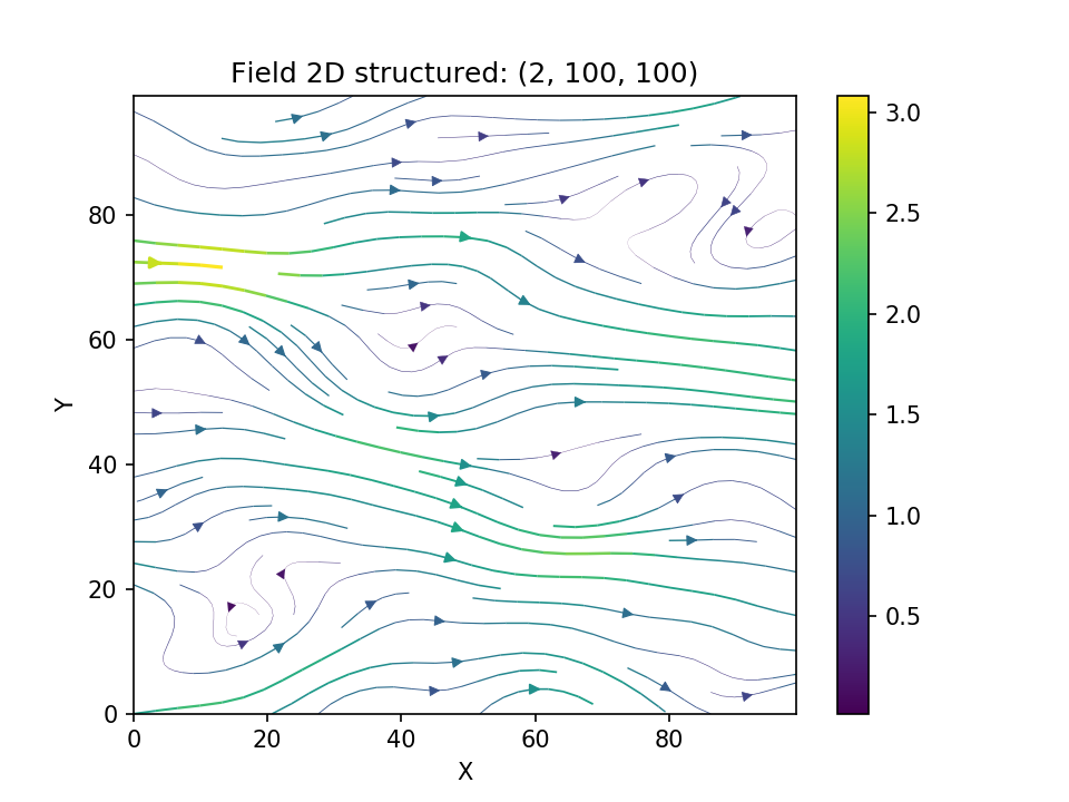
As a first example we are going to generate a vector field with a Gaussian covariance model on a structured grid:

import numpy as np
import matplotlib.pyplot as plt
from gstools import SRF, Gaussian
x = np.arange(100)
y = np.arange(100)
model = Gaussian(dim=2, var=1, len_scale=10)
srf = SRF(model, generator='VectorField')
srf((x, y), mesh_type='structured', seed=19841203)
srf.plot()

And we get a beautiful streamflow plot:

Let us have a look at the influence of the covariance model. Choosing the exponential model and keeping all other parameters the same

from gstools import Exponential

model2 = Exponential(dim=2, var=1, len_scale=10)
srf.model = model2
srf((x, y), mesh_type='structured', seed=19841203)
srf.plot()

we get following result

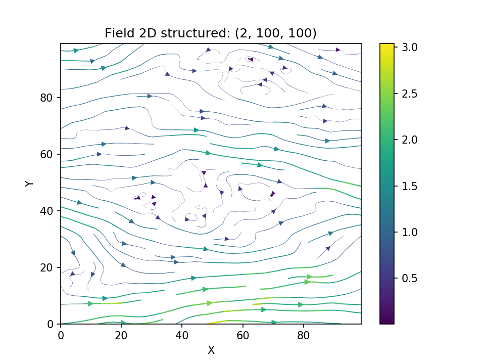
and we see, that the wiggles are much “rougher” than the smooth Gaussian ones.

Applications¶

One great advantage of the Kraichnan method is, that after some initializations, one can compute the velocity field at arbitrary points, online, with hardly any overhead. This means, that for a Lagrangian transport simulation for example, the velocity can be evaluated at each particle position very efficiently and without any interpolation. These field interpolations are a common problem for Lagrangian methods.