Tutorial 7: Field transformations
The generated fields of gstools are ordinary Gaussian random fields. In application there are several transformations to describe real world problems in an appropriate manner.
GStools provides a submodule gstools.transform with a range of
common transformations:
binary(fld[, divide, upper, lower]) |
Binary transformation. |
boxcox(fld[, lmbda, shift]) |
Box-Cox transformation. |
zinnharvey(fld[, conn]) |
Zinn and Harvey transformation to connect low or high values. |
normal_force_moments(fld) |
Force moments of a normal distributed field. |
normal_to_lognormal(fld) |
Transform normal distribution to log-normal distribution. |
normal_to_uniform(fld) |
Transform normal distribution to uniform distribution on [0, 1]. |
normal_to_arcsin(fld[, a, b]) |
Transform normal distribution to the bimodal arcsin distribution. |
normal_to_uquad(fld[, a, b]) |
Transform normal distribution to U-quadratic distribution. |
Implementation
All the transformations take a field class, that holds a generated field, as input and will manipulate this field inplace.
Simply import the transform submodule and apply a transformation to the srf class:
from gstools import transform as tf
...
tf.normal_to_lognormal(srf)
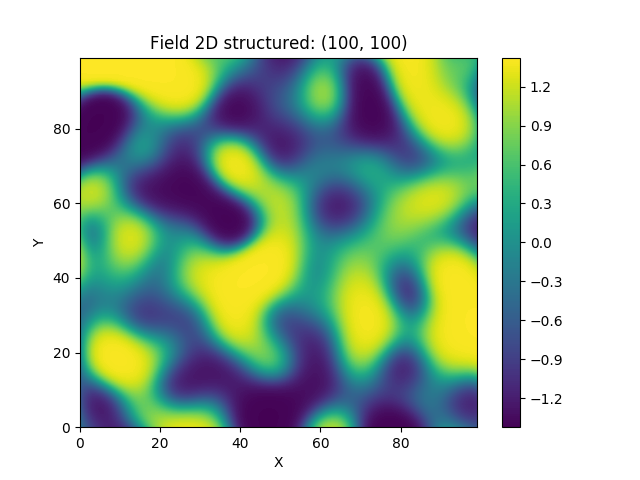
In the following we will start from a simple random field following a Gaussian covariance:
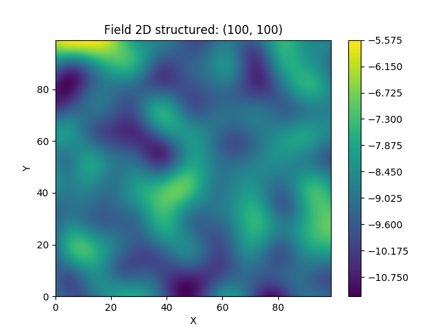
1. Example: log-normal fields
Here we transform a field to a log-normal distribution:
from gstools import SRF, Gaussian
from gstools import transform as tf
# structured field with a size of 100x100 and a grid-size of 1x1
x = y = range(100)
model = Gaussian(dim=2, var=1, len_scale=10)
srf = SRF(model, seed=20170519)
srf.structured([x, y])
tf.normal_to_lognormal(srf)
srf.plot()
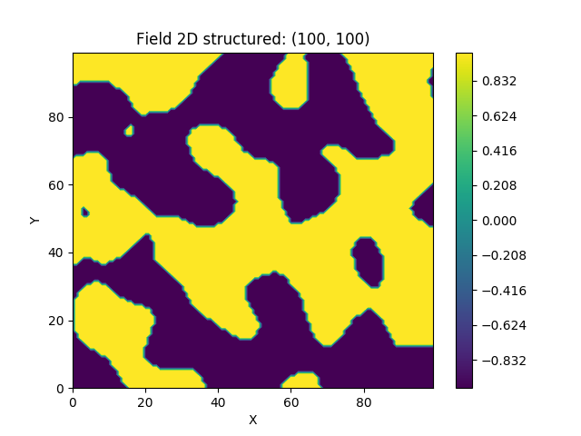
2. Example: binary fields
Here we transform a field to a binary field with only two values. The dividing value is the mean by default and the upper and lower values are derived to preserve the variance.
from gstools import SRF, Gaussian
from gstools import transform as tf
# structured field with a size of 100x100 and a grid-size of 1x1
x = y = range(100)
model = Gaussian(dim=2, var=1, len_scale=10)
srf = SRF(model, seed=20170519)
srf.structured([x, y])
tf.binary(srf)
srf.plot()
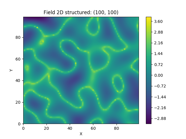
3. Example: Zinn & Harvey transformation
Here, we transform a field with the so called “Zinn & Harvey” transformation presented in Zinn & Harvey (2003). With this transformation, one could overcome the restriction that in ordinary Gaussian random fields the mean values are the ones being the most connected.
from gstools import SRF, Gaussian
from gstools import transform as tf
# structured field with a size of 100x100 and a grid-size of 1x1
x = y = range(100)
model = Gaussian(dim=2, var=1, len_scale=10)
srf = SRF(model, seed=20170519)
srf.structured([x, y])
tf.zinnharvey(srf, conn="high")
srf.plot()
4. Example: bimodal fields
We provide two transformations to obtain bimodal distributions:
Both transformations will preserve the mean and variance of the given field by default.
from gstools import SRF, Gaussian
from gstools import transform as tf
# structured field with a size of 100x100 and a grid-size of 1x1
x = y = range(100)
model = Gaussian(dim=2, var=1, len_scale=10)
srf = SRF(model, seed=20170519)
field = srf.structured([x, y])
tf.normal_to_arcsin(srf)
srf.plot()
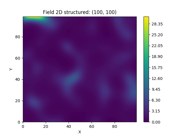
5. Example: Combinations
You can combine different transformations simply by successively applying them.
Here, we first force the single field realization to hold the given moments, namely mean and variance. Then we apply the Zinn & Harvey transformation to connect the low values. Afterwards the field is transformed to a binary field and last but not least, we transform it to log-values.
from gstools import SRF, Gaussian
from gstools import transform as tf
# structured field with a size of 100x100 and a grid-size of 1x1
x = y = range(100)
model = Gaussian(dim=2, var=1, len_scale=10)
srf = SRF(model, mean=-9, seed=20170519)
srf.structured([x, y])
tf.normal_force_moments(srf)
tf.zinnharvey(srf, conn="low")
tf.binary(srf)
tf.normal_to_lognormal(srf)
srf.plot()
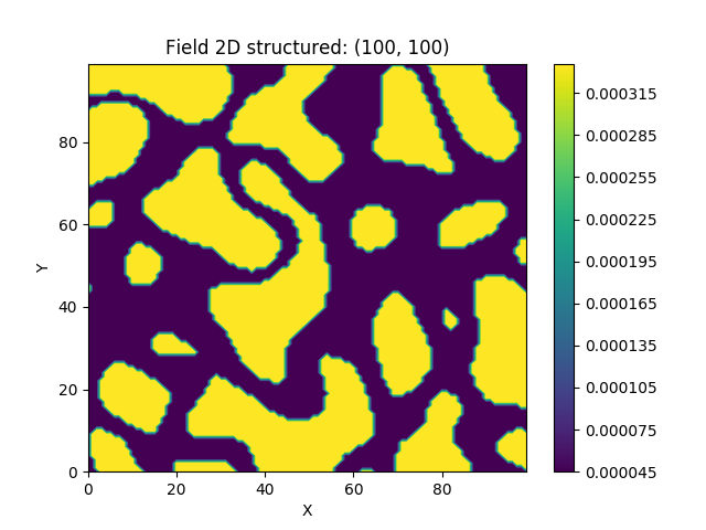
The resulting field could be interpreted as a transmissivity field, where the values of low permeability are the ones being the most connected and only two kinds of soil exist.