Truncated Power Law Variograms¶

GSTools also implements truncated power law variograms, which can be represented as a superposition of scale dependant modes in form of standard variograms, which are truncated by a lower- $\ell_{\mathrm{low}}$ and an upper length-scale $\ell_{\mathrm{up}}$ .

This example shows the truncated power law (TPLStable) based on the Stable covariance model and is given by

$\gamma_{\ell_{\mathrm{low}},\ell_{\mathrm{up}}}(r) = \intop_{\ell_{\mathrm{low}}}^{\ell_{\mathrm{up}}} \gamma(r,\lambda) \frac{\rm d \lambda}{\lambda}$

with Stable modes on each scale:

$\gamma(r,\lambda) &= \sigma^2(\lambda)\cdot\left(1- \exp\left[- \left(\frac{r}{\lambda}\right)^{\alpha}\right] \right)\\ \sigma^2(\lambda) &= C\cdot\lambda^{2H}$

which gives Gaussian modes for alpha=2 or Exponential modes for alpha=1.

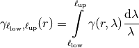
For $\ell_{\mathrm{low}}=0$ this results in:

$\gamma_{\ell_{\mathrm{up}}}(r) &= \sigma^2_{\ell_{\mathrm{up}}}\cdot\left(1- \frac{2H}{\alpha} \cdot E_{1+\frac{2H}{\alpha}} \left[\left(\frac{r}{\ell_{\mathrm{up}}}\right)^{\alpha}\right] \right) \\ \sigma^2_{\ell_{\mathrm{up}}} &= C\cdot\frac{\ell_{\mathrm{up}}^{2H}}{2H}$

import numpy as np
import gstools as gs

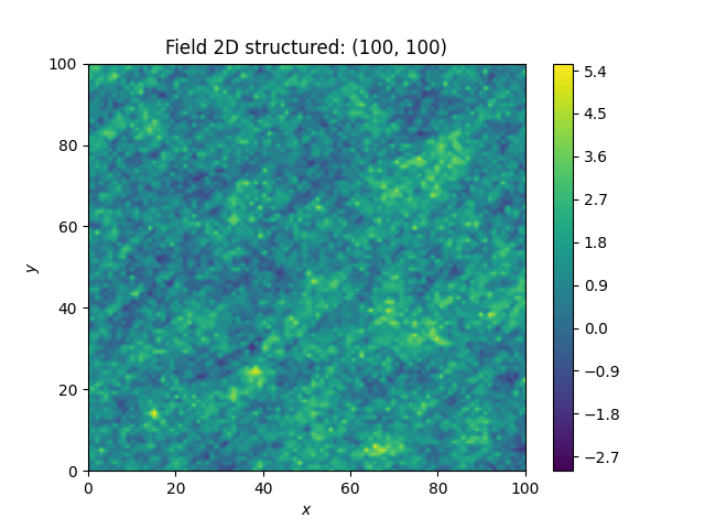
x = y = np.linspace(0, 100, 100)
model = gs.TPLStable(
    dim=2,  # spatial dimension
    var=1,  # variance (C is calculated internally, so variance is actually 1)
    len_low=0,  # lower truncation of the power law
    len_scale=10,  # length scale (a.k.a. range), len_up = len_low + len_scale
    nugget=0.1,  # nugget
    anis=0.5,  # anisotropy between main direction and transversal ones
    angles=np.pi / 4,  # rotation angles
    alpha=1.5,  # shape parameter from the stable model
    hurst=0.7,  # hurst coefficient from the power law
)
srf = gs.SRF(model, mean=1.0, seed=19970221)
srf.structured([x, y])
srf.plot()

Total running time of the script: ( 0 minutes 15.190 seconds)

Gallery generated by Sphinx-Gallery