Simple Kriging¶

Simple kriging assumes a known mean of the data. For simplicity we assume a mean of 0, which can be achieved by subtracting the mean from the observed values and subsequently adding it to the resulting data.

The resulting equation system for $W$ is given by:

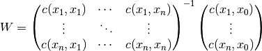
$W = \begin{pmatrix}c(x_1,x_1) & \cdots & c(x_1,x_n) \\ \vdots & \ddots & \vdots \\ c(x_n,x_1) & \cdots & c(x_n,x_n) \end{pmatrix}^{-1} \begin{pmatrix}c(x_1,x_0) \\ \vdots \\ c(x_n,x_0) \end{pmatrix}$

Thereby $c(x_i,x_j)$ is the covariance of the given observations.

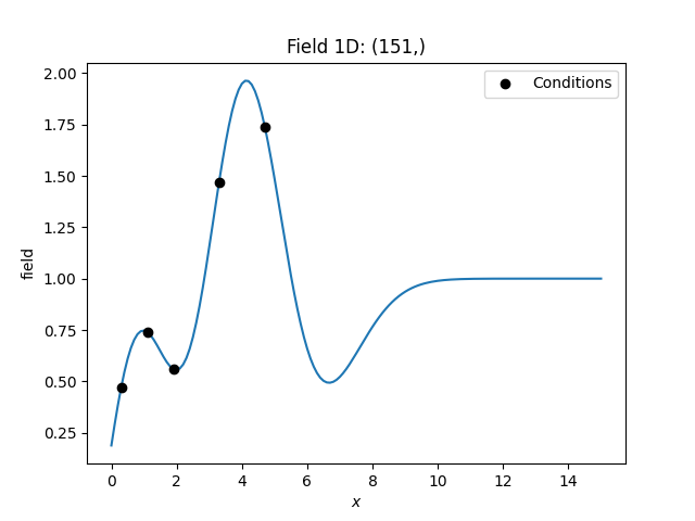
Example¶

Here we use simple kriging in 1D (for plotting reasons) with 5 given observations/conditions. The mean of the field has to be given beforehand.

import numpy as np
from gstools import Gaussian, krige

# condtions
cond_pos = [0.3, 1.9, 1.1, 3.3, 4.7]
cond_val = [0.47, 0.56, 0.74, 1.47, 1.74]
# resulting grid
gridx = np.linspace(0.0, 15.0, 151)
# spatial random field class
model = Gaussian(dim=1, var=0.5, len_scale=2)

krig = krige.Simple(model, mean=1, cond_pos=cond_pos, cond_val=cond_val)
krig(gridx)

ax = krig.plot()
ax.scatter(cond_pos, cond_val, color="k", zorder=10, label="Conditions")
ax.legend()

Total running time of the script: ( 0 minutes 0.110 seconds)

Gallery generated by Sphinx-Gallery