Note
Click here to download the full example code
Ordinary Kriging
Ordinary kriging will estimate an appropriate mean of the field, based on the given observations/conditions and the covariance model used.
The resulting system of equations for  is given by:
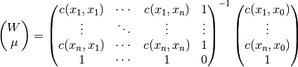
Thereby  is the covariance of the given observations
and
is the covariance of the given observations
and  is a Lagrange multiplier to minimize the kriging error and estimate the mean.
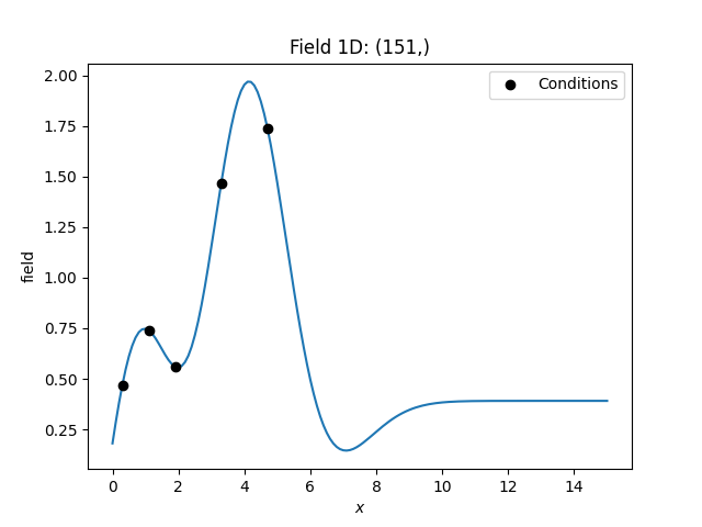
Example
Here we use ordinary kriging in 1D (for plotting reasons) with 5 given observations/conditions.
The estimated mean can be accessed by krig.mean.
import numpy as np
from gstools import Gaussian, krige

# condtions
cond_pos = [0.3, 1.9, 1.1, 3.3, 4.7]
cond_val = [0.47, 0.56, 0.74, 1.47, 1.74]
# resulting grid
gridx = np.linspace(0.0, 15.0, 151)
# spatial random field class
model = Gaussian(dim=1, var=0.5, len_scale=2)
krig = krige.Ordinary(model, cond_pos=cond_pos, cond_val=cond_val)
krig(gridx)
ax = krig.plot()
ax.scatter(cond_pos, cond_val, color="k", zorder=10, label="Conditions")
ax.legend()
Total running time of the script: ( 0 minutes 0.107 seconds)