Creating an Ensemble of conditioned 2D Fields

Let’s create an ensemble of conditioned random fields in 2D.

import numpy as np
import matplotlib.pyplot as plt
import gstools as gs


# conditioning data (x, y, value)
cond_pos = [[0.3, 1.9, 1.1, 3.3, 4.7], [1.2, 0.6, 3.2, 4.4, 3.8]]
cond_val = [0.47, 0.56, 0.74, 1.47, 1.74]

# grid definition for output field
x = np.arange(0, 5, 0.1)
y = np.arange(0, 5, 0.1)

model = gs.Gaussian(dim=2, var=0.5, len_scale=5, anis=0.5, angles=-0.5)
krige = gs.Krige(model, cond_pos=cond_pos, cond_val=cond_val)
cond_srf = gs.CondSRF(krige)

We create a list containing the generated conditioned fields.

ens_no = 4
field = []
for i in range(ens_no):
    field.append(cond_srf.structured([x, y], seed=i))

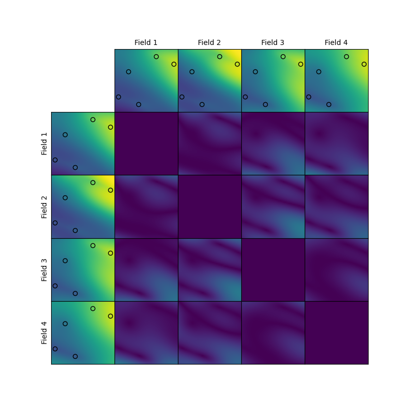
Now let’s have a look at the pairwise differences between the generated fields. We will see, that they coincide at the given conditions.

fig, ax = plt.subplots(ens_no + 1, ens_no + 1, figsize=(8, 8))
# plotting kwargs for scatter and image
sc_kwargs = dict(c=cond_val, edgecolors="k", vmin=0, vmax=np.max(field))
im_kwargs = dict(extent=2 * [0, 5], origin="lower", vmin=0, vmax=np.max(field))
for i in range(ens_no):
    # conditioned fields and conditions
    ax[i + 1, 0].imshow(field[i].T, **im_kwargs)
    ax[i + 1, 0].scatter(*cond_pos, **sc_kwargs)
    ax[i + 1, 0].set_ylabel(f"Field {i+1}", fontsize=10)
    ax[0, i + 1].imshow(field[i].T, **im_kwargs)
    ax[0, i + 1].scatter(*cond_pos, **sc_kwargs)
    ax[0, i + 1].set_title(f"Field {i+1}", fontsize=10)
    # absolute differences
    for j in range(ens_no):
        ax[i + 1, j + 1].imshow(np.abs(field[i] - field[j]).T, **im_kwargs)

# beautify plots
ax[0, 0].axis("off")
for a in ax.flatten():
    a.set_xticklabels([]), a.set_yticklabels([])
    a.set_xticks([]), a.set_yticks([])
fig.subplots_adjust(wspace=0, hspace=0)
fig.show()