Intrinsic Collocated Cokriging

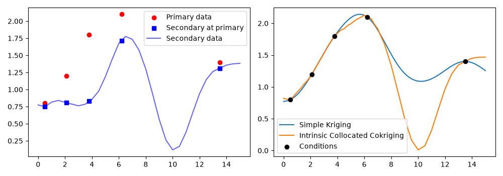
Intrinsic Collocated Cokriging (ICCK) improves variance estimation compared to Simple Collocated Cokriging.

This example demonstrates the correlogram-based API using MarkovModel1.

The variance formula is:

\[\sigma^2_{ICCK} = (1 - \rho_0^2) \cdot \sigma^2_{SK}\]

Example

Here we compare Simple Kriging with Intrinsic Collocated Cokriging using the MarkovModel1 correlogram.

import matplotlib.pyplot as plt
import numpy as np

from gstools import Gaussian, MarkovModel1, krige
from gstools.cokriging import IntrinsicCollocated

# condtions
np.random.seed(4)
cond_pos = np.array([0.5, 2.1, 3.8, 6.2, 13.5])
cond_val = np.array([0.8, 1.2, 1.8, 2.1, 1.4])
gridx = np.linspace(0.0, 15.0, 151)
model = Gaussian(dim=1, var=0.5, len_scale=2.0)

Generate correlated secondary data

sec_pos = np.linspace(0, 15, 31)
primary_trend = np.interp(sec_pos, cond_pos, cond_val)
gap_feature = -1.6 * np.exp(-(((sec_pos - 10.0) / 2.0) ** 2))
gap_feature2 = -0.95 * np.exp(-(((sec_pos - 4.0) / 2.0) ** 2))
sec_val = 0.99 * primary_trend + gap_feature + gap_feature2

sec_grid = np.interp(gridx, sec_pos, sec_val)
sec_at_primary = np.interp(cond_pos, sec_pos, sec_val)

Simple Kriging and Intrinsic Collocated Cokriging

sk = krige.Simple(model, cond_pos=cond_pos, cond_val=cond_val, mean=1.0)
sk_field, sk_var = sk(gridx, return_var=True)

# Compute cross-correlation from data
cross_corr = np.corrcoef(cond_val, sec_at_primary)[0, 1]

# Create MarkovModel1 correlogram
correlogram = MarkovModel1(
    primary_model=model,
    cross_corr=cross_corr,
    secondary_var=np.var(sec_val),
    primary_mean=1.0,
    secondary_mean=np.mean(sec_val),
)

# Intrinsic Collocated Cokriging
icck = IntrinsicCollocated(
    correlogram,
    cond_pos=cond_pos,
    cond_val=cond_val,
    secondary_cond_pos=cond_pos,
    secondary_cond_val=sec_at_primary,
)
icck_field, icck_var = icck(gridx, secondary_data=sec_grid, return_var=True)

fig, ax = plt.subplots(1, 2, figsize=(10, 3.5))

ax[0].scatter(cond_pos, cond_val, color="red", label="Primary data")
ax[0].scatter(
    cond_pos,
    sec_at_primary,
    color="blue",
    marker="s",
    label="Secondary at primary",
)
ax[0].plot(sec_pos, sec_val, "b-", alpha=0.6, label="Secondary data")
ax[0].legend()

ax[1].plot(gridx, sk_field, label="Simple Kriging")
ax[1].plot(gridx, icck_field, label="Intrinsic Collocated Cokriging")
ax[1].scatter(cond_pos, cond_val, color="k", zorder=10, label="Conditions")
ax[1].legend()

plt.tight_layout()
plt.show()