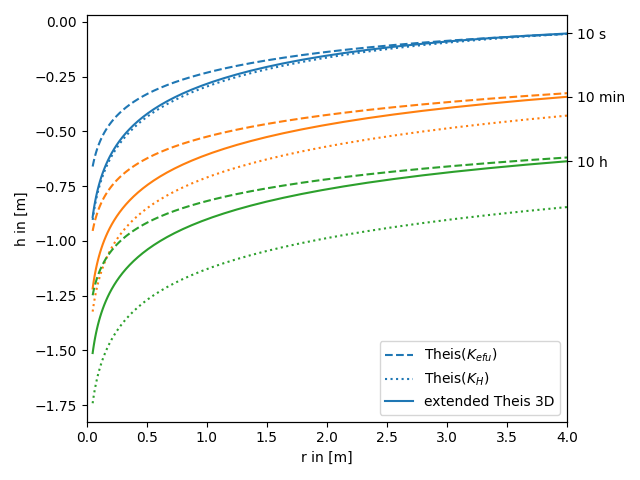
The extended Theis solution in 3D

We provide an extended theis solution, that incorporates the effectes of a heterogeneous conductivity field on a pumping test. It also includes an anisotropy ratio of the horizontal and vertical length scales.

In the following this extended solution is compared to the standard theis solution for well flow. You can nicely see, that the extended solution represents a transition between the theis solutions for the effective and harmonic-mean conductivity.

Reference: Müller 2015

import numpy as np
from matplotlib import pyplot as plt

from anaflow import ext_theis_3d, theis
from anaflow.tools.special import aniso

We use three time steps: 10s, 10min, 10h

time_labels = ["10 s", "10 min", "10 h"]
time = [10, 600, 36000]  # 10s, 10min, 10h

Radius from the pumping well should be in [0, 4].

rad = np.geomspace(0.05, 4)

Parameters of heterogeneity, storage, extend and pumping rate.

var = 0.5  # variance of the log-conductivity
len_scale = 10.0  # correlation length of the log-conductivity
anis = 0.75  # anisotropy ratio of the log-conductivity
KG = 1e-4  # the geometric mean of the conductivity
Kefu = KG * np.exp(
    var * (0.5 - aniso(anis))
)  # the effective conductivity for uniform flow
KH = KG * np.exp(-var / 2.0)  # the harmonic mean of the conductivity

S = 1e-4  # storage
L = 1.0  # vertical extend of the aquifer
rate = -1e-4  # pumping rate

Now let’s compare the extended Theis solution to the classical solutions for the near and far field values of transmissivity.

head_Kefu = theis(time, rad, S, Kefu * L, rate)
head_KH = theis(time, rad, S, KH * L, rate)
head_ef = ext_theis_3d(time, rad, S, KG, var, len_scale, anis, L, rate)
time_ticks = []
for i, step in enumerate(time):
    label_TG = "Theis($K_{efu}$)" if i == 0 else None
    label_TH = "Theis($K_H$)" if i == 0 else None
    label_ef = "extended Theis 3D" if i == 0 else None
    plt.plot(
        rad, head_Kefu[i], label=label_TG, color="C" + str(i), linestyle="--"
    )
    plt.plot(
        rad, head_KH[i], label=label_TH, color="C" + str(i), linestyle=":"
    )
    plt.plot(rad, head_ef[i], label=label_ef, color="C" + str(i))
    time_ticks.append(head_ef[i][-1])

plt.xlabel("r in [m]")
plt.ylabel("h in [m]")
plt.legend()
ylim = plt.gca().get_ylim()
plt.gca().set_xlim([0, rad[-1]])
ax2 = plt.gca().twinx()
ax2.set_yticks(time_ticks)
ax2.set_yticklabels(time_labels)
ax2.set_ylim(ylim)
plt.tight_layout()
plt.show()