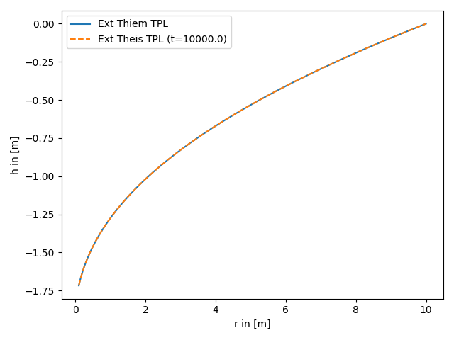
Convergence of the extended Theis solutions for truncated power laws

Here we set an outer boundary to the transient solution, so this condition coincides with the references head of the steady solution.

Reference: (not yet published)

import numpy as np
from matplotlib import pyplot as plt

from anaflow import ext_theis_tpl, ext_thiem_tpl

time = 1e4  # time point for steady state
rad = np.geomspace(0.1, 10)  # radius from the pumping well in [0, 4]
r_ref = 10.0  # reference radius

KG = 1e-4  # the geometric mean of the transmissivity
len_scale = 5.0  # correlation length of the log-transmissivity
hurst = 0.5  # hurst coefficient
var = 0.5  # variance of the log-transmissivity
dim = 1.5  # using a fractional dimension

S = 1e-4  # storativity
rate = -1e-4  # pumping rate

head1 = ext_thiem_tpl(
    rad, r_ref, KG, len_scale, hurst, var, dim=dim, rate=rate
)
head2 = ext_theis_tpl(
    time, rad, S, KG, len_scale, hurst, var, dim=dim, rate=rate, r_bound=r_ref
)

plt.plot(rad, head1, label="Ext Thiem TPL")
plt.plot(rad, head2, label="Ext Theis TPL (t={})".format(time), linestyle="--")

plt.xlabel("r in [m]")
plt.ylabel("h in [m]")
plt.legend()
plt.tight_layout()
plt.show()