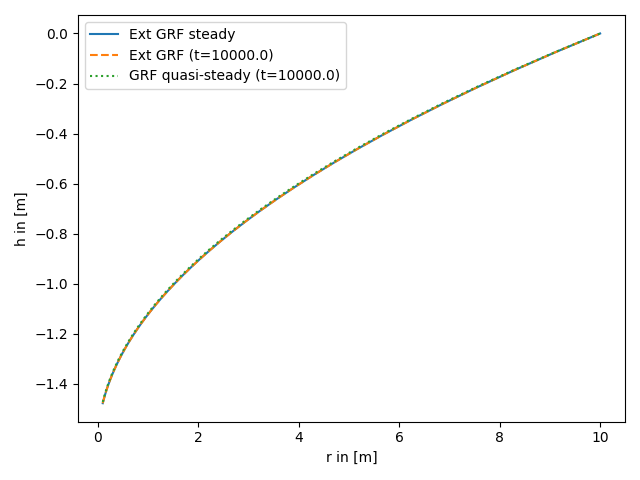
Convergence of the general radial flow model (GRF)

The GRF model introduces an arbitrary flow dimension and was presented to analyze groundwater flow in rock formations. In the following we compare the bounded transient solution for late times, the unbounded quasi steady solution and the steady state.

Reference: Barker 1988

import numpy as np
from matplotlib import pyplot as plt

from anaflow import ext_grf, ext_grf_steady, grf

time = 1e4  # time point for steady state
rad = np.geomspace(0.1, 10)  # radius from the pumping well in [0, 4]
r_ref = 10.0  # reference radius

K = 1e-4  # the geometric mean of the transmissivity
dim = 1.5  # using a fractional dimension

rate = -1e-4  # pumping rate

head1 = ext_grf_steady(rad, r_ref, K, dim=dim, rate=rate)
head2 = ext_grf(time, rad, [1e-4], [K], [0, r_ref], dim=dim, rate=rate)
head3 = grf(time, rad, 1e-4, K, dim=dim, rate=rate)
head3 -= head3[-1]  # quasi-steady

plt.plot(rad, head1, label="Ext GRF steady")
plt.plot(rad, head2, label="Ext GRF (t={})".format(time), linestyle="--")
plt.plot(
    rad, head3, label="GRF quasi-steady (t={})".format(time), linestyle=":"
)

plt.xlabel("r in [m]")
plt.ylabel("h in [m]")
plt.legend()
plt.tight_layout()
plt.show()