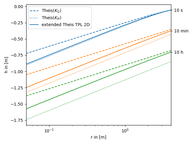
The extended Theis solution for truncated power laws

We provide an extended theis solution, that incorporates the effectes of a heterogeneous conductivity field following a truncated power law. In addition, it incorporates the assumptions of the general radial flow model and provides an arbitrary flow dimension.

In the following this extended solution is compared to the standard theis solution for well flow. You can nicely see, that the extended solution represents a transition between the theis solutions for the well- and farfield-conductivity.

Reference: (not yet published)

import numpy as np
from matplotlib import pyplot as plt

from anaflow import ext_theis_tpl, theis

We use three time steps: 10s, 10min, 10h

time_labels = ["10 s", "10 min", "10 h"]
time = [10, 600, 36000]  # 10s, 10min, 10h

Radius from the pumping well should be in [0, 4].

rad = np.geomspace(0.05, 4)

Parameters of heterogeneity, storage and pumping rate.

var = 0.5  # variance of the log-conductivity
len_scale = 20.0  # upper bound for the length scale
hurst = 0.5  # hurst coefficient
KG = 1e-4  # the geometric mean of the conductivity
KH = KG * np.exp(-var / 2)  # the harmonic mean of the conductivity

S = 1e-4  # storage
rate = -1e-4  # pumping rate

Now let’s compare the extended Theis TPL solution to the classical solutions for the near and far field values of transmissivity.

head_KG = theis(time, rad, S, KG, rate)
head_KH = theis(time, rad, S, KH, rate)
head_ef = ext_theis_tpl(
    time=time,
    rad=rad,
    storage=S,
    cond_gmean=KG,
    len_scale=len_scale,
    hurst=hurst,
    var=var,
    rate=rate,
)
time_ticks = []
for i, step in enumerate(time):
    label_TG = "Theis($K_G$)" if i == 0 else None
    label_TH = "Theis($K_H$)" if i == 0 else None
    label_ef = "extended Theis TPL 2D" if i == 0 else None
    plt.plot(rad, head_KG[i], label=label_TG, color="C" + str(i), linestyle="--")
    plt.plot(rad, head_KH[i], label=label_TH, color="C" + str(i), linestyle=":")
    plt.plot(rad, head_ef[i], label=label_ef, color="C" + str(i))
    time_ticks.append(head_ef[i][-1])

plt.xscale("log")
plt.xlabel("r in [m]")
plt.ylabel("h in [m]")
plt.legend()
ylim = plt.gca().get_ylim()
plt.gca().set_xlim([rad[0], rad[-1]])
ax2 = plt.gca().twinx()
ax2.set_yticks(time_ticks)
ax2.set_yticklabels(time_labels)
ax2.set_ylim(ylim)
plt.tight_layout()
plt.show()