Note
Go to the end to download the full example code.
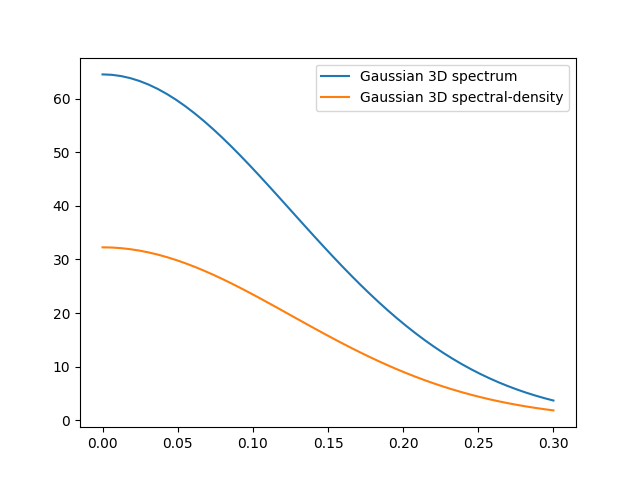
Spectral methods
The spectrum of a covariance model is given by:
Since the covariance function \(C(r)\) is radially symmetric, we can calculate this by the hankel-transformation:
Where \(k=\left\Vert\mathbf{k}\right\Vert\).
Depending on the spectrum, the spectral-density is defined by:
You can access these methods by:
Note
The spectral-density is given by the radius of the input phase. But it is
not a probability density function for the radius of the phase.
To obtain the pdf for the phase-radius, you can use the methods
CovModel.spectral_rad_pdf
or CovModel.ln_spectral_rad_pdf for the logarithm.
The user can also provide a cdf (cumulative distribution function) by
defining a method called spectral_rad_cdf
and/or a ppf (percent-point function)
by spectral_rad_ppf.
The attributes CovModel.has_cdf
and CovModel.has_ppf will check for that.
Total running time of the script: (0 minutes 0.043 seconds)