Note
Go to the end to download the full example code.
Automatic binning with lat-lon data
In this example we demonstrate automatic binning for a tiny data set containing temperature records from Germany (See the detailed DWD example for more information on the data).
We use a data set from 20 meteo-stations choosen randomly.
import numpy as np

import gstools as gs

# lat, lon, temperature
data = np.array(
    [
        [52.9336, 8.237, 15.7],
        [48.6159, 13.0506, 13.9],
        [52.4853, 7.9126, 15.1],
        [50.7446, 9.345, 17.0],
        [52.9437, 12.8518, 21.9],
        [53.8633, 8.1275, 11.9],
        [47.8342, 10.8667, 11.4],
        [51.0881, 12.9326, 17.2],
        [48.406, 11.3117, 12.9],
        [49.7273, 8.1164, 17.2],
        [49.4691, 11.8546, 13.4],
        [48.0197, 12.2925, 13.9],
        [50.4237, 7.4202, 18.1],
        [53.0316, 13.9908, 21.3],
        [53.8412, 13.6846, 21.3],
        [54.6792, 13.4343, 17.4],
        [49.9694, 9.9114, 18.6],
        [51.3745, 11.292, 20.2],
        [47.8774, 11.3643, 12.7],
        [50.5908, 12.7139, 15.8],
    ]
)
pos = data.T[:2]  # lat, lon
field = data.T[2]  # temperature
Since the overall range of these meteo-stations is too low, we can use the data-variance as additional information during the fit of the variogram.
emp_v = gs.vario_estimate(pos, field, latlon=True, geo_scale=gs.KM_SCALE)
sph = gs.Spherical(latlon=True, geo_scale=gs.KM_SCALE)
sph.fit_variogram(*emp_v, sill=np.var(field))
ax = sph.plot("vario_yadrenko", x_max=2 * np.max(emp_v[0]))
ax.scatter(*emp_v, label="Empirical variogram")
ax.legend()
print(sph)
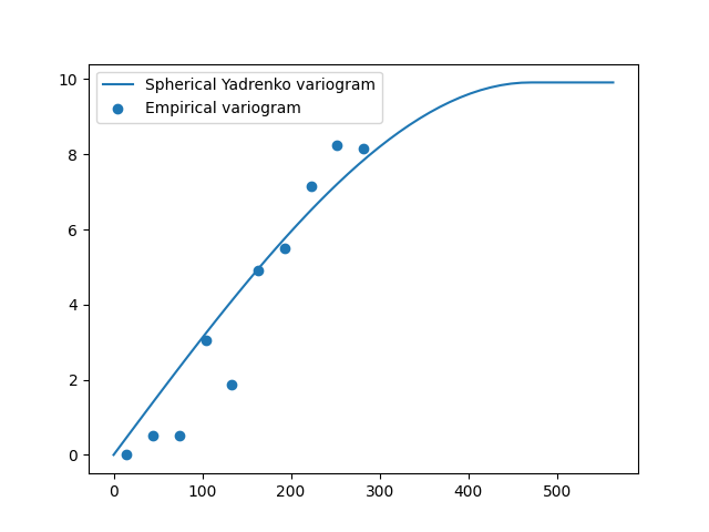
Spherical(latlon=True, var=9.91, len_scale=4.7e+02, geo_scale=6.37e+03)
As we can see, the variogram fitting was successful and providing the data variance helped finding the right length-scale.
Now, we’ll use this covariance model to interpolate the given data with ordinary kriging.
# enclosing box for data points
grid_lat = np.linspace(np.min(pos[0]), np.max(pos[0]))
grid_lon = np.linspace(np.min(pos[1]), np.max(pos[1]))
# ordinary kriging
krige = gs.krige.Ordinary(sph, pos, field)
krige((grid_lat, grid_lon), mesh_type="structured")
ax = krige.plot()
# plotting lat on y-axis and lon on x-axis
ax.scatter(pos[1], pos[0], 50, c=field, edgecolors="k", label="input")
ax.legend()
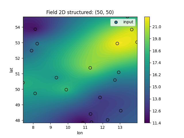
Looks good, doesn’t it?
This workflow is also implemented in the Krige class, by setting
fit_variogram=True. Then the whole procedure shortens:
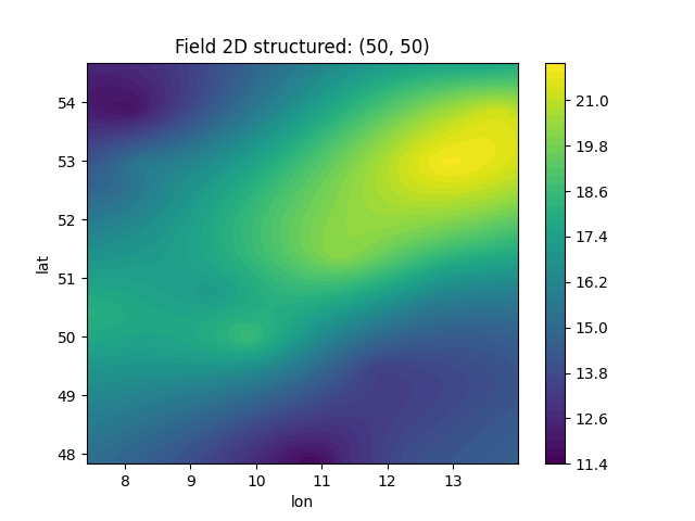
Spherical(latlon=True, var=9.91, len_scale=4.7e+02, geo_scale=6.37e+03)
This example shows, that setting up variogram estimation and kriging routines is straight forward with GSTools!
Total running time of the script: (0 minutes 0.215 seconds)