The Covariance Model
One of the core-features of GSTools is the powerful CovModel
class, which allows you to easily define arbitrary covariance models by
yourself. The resulting models provide a bunch of nice features to explore the
covariance models.
A covariance model is used to characterize the semi-variogram, denoted by \(\gamma\), of a spatial random field. In GSTools, we use the following form for an isotropic and stationary field:
Where:
\(r\) is the lag distance
\(\ell\) is the main correlation length
\(s\) is a scaling factor for unit conversion or normalization
\(\sigma^2\) is the variance
\(n\) is the nugget (subscale variance)
\(\mathrm{cor}(h)\) is the normalized correlation function depending on the non-dimensional distance \(h=s\cdot\frac{r}{\ell}\)
Depending on the normalized correlation function, all covariance models in GSTools are providing the following functions:
\(\rho(r)=\mathrm{cor}\left(s\cdot\frac{r}{\ell}\right)\) is the so called correlation function
\(C(r)=\sigma^2\cdot\rho(r)\) is the so called covariance function, which gives the name for our GSTools class
Note
We are not limited to isotropic models. GSTools supports anisotropy ratios for length scales in orthogonal transversal directions like:
\(x_0\) (main direction)
\(x_1\) (1. transversal direction)
\(x_2\) (2. transversal direction)
…
These main directions can also be rotated. Just have a look at the corresponding examples.
Provided Covariance Models
The following standard covariance models are provided by GSTools
|
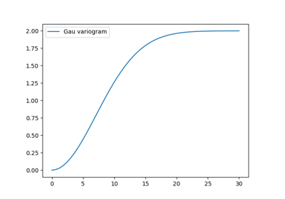
The Gaussian covariance model. |
|
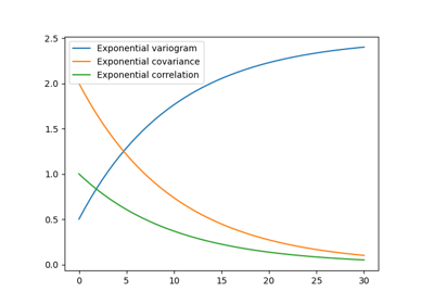
The Exponential covariance model. |
|
The Matérn covariance model. |
|
The Exponential Integral covariance model. |
|
The stable covariance model. |
|
The rational quadratic covariance model. |
|
The Cubic covariance model. |
|
The bounded linear covariance model. |
|
The circular covariance model. |
|
The Spherical covariance model. |
|
The Hyper-Spherical covariance model. |
|
The Super-Spherical covariance model. |
|
The J-Bessel hole model. |
|
The simply truncated power law model. |
As a special feature, we also provide truncated power law (TPL) covariance models
|
Truncated-Power-Law with Gaussian modes. |
|
Truncated-Power-Law with Exponential modes. |
|
Truncated-Power-Law with Stable modes. |
These models provide a lower and upper length scale truncation for superpositioned models.