Note
Go to the end to download the full example code
Directional variogram estimation and fitting in 2D
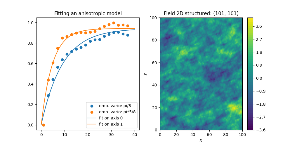
In this example, we demonstrate how to estimate a directional variogram by setting the direction angles in 2D.
Afterwards we will fit a model to this estimated variogram and show the result.
import numpy as np
from matplotlib import pyplot as plt

import gstools as gs
Generating synthetic field with anisotropy and a rotation of 22.5 degree.
angle = np.pi / 8
model = gs.Exponential(dim=2, len_scale=[10, 5], angles=angle)
x = y = range(101)
srf = gs.SRF(model, seed=123456)
field = srf((x, y), mesh_type="structured")
Now we are going to estimate a directional variogram with an angular tolerance of 11.25 degree and a bandwith of 8.
bins = range(0, 40, 2)
bin_center, dir_vario, counts = gs.vario_estimate(
    *((x, y), field, bins),
    direction=gs.rotated_main_axes(dim=2, angles=angle),
    angles_tol=np.pi / 16,
    bandwidth=8,
    mesh_type="structured",
    return_counts=True,
)
Afterwards we can use the estimated variogram to fit a model to it:
print("Original:")
print(model)
model.fit_variogram(bin_center, dir_vario)
print("Fitted:")
print(model)
Original:
Exponential(dim=2, var=1.0, len_scale=10.0, nugget=0.0, anis=[0.5], angles=[0.393])
Fitted:
Exponential(dim=2, var=0.942, len_scale=9.14, nugget=1.1e-17, anis=[0.529], angles=[0.393])
Plotting.
fig, (ax1, ax2) = plt.subplots(1, 2, figsize=[10, 5])

ax1.scatter(bin_center, dir_vario[0], label="emp. vario: pi/8")
ax1.scatter(bin_center, dir_vario[1], label="emp. vario: pi*5/8")
ax1.legend(loc="lower right")

model.plot("vario_axis", axis=0, ax=ax1, x_max=40, label="fit on axis 0")
model.plot("vario_axis", axis=1, ax=ax1, x_max=40, label="fit on axis 1")
ax1.set_title("Fitting an anisotropic model")

srf.plot(ax=ax2)
plt.show()

Without fitting a model, we see that the correlation length in the main direction is greater than the transversal one.
Total running time of the script: ( 0 minutes 8.131 seconds)