Note
Go to the end to download the full example code.
Automatic fitting
In order to demonstrate how to automatically fit normalizer and variograms, we generate synthetic log-normal data, that should be interpolated with ordinary kriging.
Normalizers are fitted by minimizing the likelihood function and variograms are fitted by estimating the empirical variogram with automatic binning and fitting the theoretical model to it. Thereby the sill is constrained to match the field variance.
Artificial data
Here we generate log-normal data following a Gaussian covariance model. We will generate the “original” field on a 60x60 mesh, from which we will take samples in order to pretend a situation of data-scarcity.
import matplotlib.pyplot as plt
import numpy as np

import gstools as gs

# structured field with edge length of 50
x = y = range(51)
pos = gs.generate_grid([x, y])
model = gs.Gaussian(dim=2, var=1, len_scale=10)
srf = gs.SRF(model, seed=20170519, normalizer=gs.normalizer.LogNormal())
# generate the original field
srf(pos)
Here, we sample 60 points and set the conditioning points and values.
Fitting and Interpolation
Now we want to interpolate the “measured” samples and we want to normalize the given data with the BoxCox transformation.
Here we set up the kriging routine and use a Stable model, that should
be fitted automatically to the given data
and we pass the BoxCox normalizer in order to gain normality.
The normalizer will be fitted automatically to the data,
by setting fit_normalizer=True.
The covariance/variogram model will be fitted by an automatic workflow
by setting fit_variogram=True.
First, let’s have a look at the fitting results:
print(krige.model)
print(krige.normalizer)
Stable(dim=2, var=0.576, len_scale=8.85, nugget=0.00682, alpha=2.0)
BoxCox(lmbda=-0.0754)
As we see, it went quite well. Variance is a bit underestimated, but length scale and nugget are good. The shape parameter of the stable model is correctly estimated to be close to 2, so we result in a Gaussian like model.
The BoxCox parameter lmbda was estimated to be almost 0, which means, the log-normal distribution was correctly fitted.
Now let’s run the kriging interpolation.
krige(pos)
Plotting
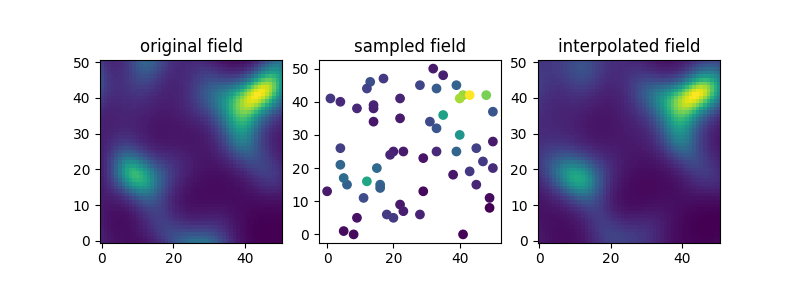
Finally let’s compare the original, sampled and interpolated fields. As we’ll see, there is a lot of information in the covariance structure of the measurement samples and the field is reconstructed quite accurately.
fig, ax = plt.subplots(1, 3, figsize=[8, 3])
ax[0].imshow(srf.field.reshape(len(x), len(y)).T, origin="lower")
ax[1].scatter(*cond_pos, c=cond_val)
ax[2].imshow(krige.field.reshape(len(x), len(y)).T, origin="lower")
# titles
ax[0].set_title("original field")
ax[1].set_title("sampled field")
ax[2].set_title("interpolated field")
# set aspect ratio to equal in all plots
[ax[i].set_aspect("equal") for i in range(3)]
Total running time of the script: (0 minutes 0.184 seconds)