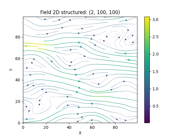
Generating a Random 2D Vector Field

As a first example we are going to generate a 2d vector field with a Gaussian covariance model on a structured grid:

import numpy as np

import gstools as gs

# the grid
x = np.arange(100)
y = np.arange(100)

# a smooth Gaussian covariance model
model = gs.Gaussian(dim=2, var=1, len_scale=10)
srf = gs.SRF(model, generator="VectorField", seed=19841203)
srf((x, y), mesh_type="structured")
srf.plot()

Let us have a look at the influence of the covariance model. Choosing the exponential model and keeping all other parameters the same

# a rougher exponential covariance model
model2 = gs.Exponential(dim=2, var=1, len_scale=10)
srf.model = model2
srf((x, y), mesh_type="structured", seed=19841203)
srf.plot()

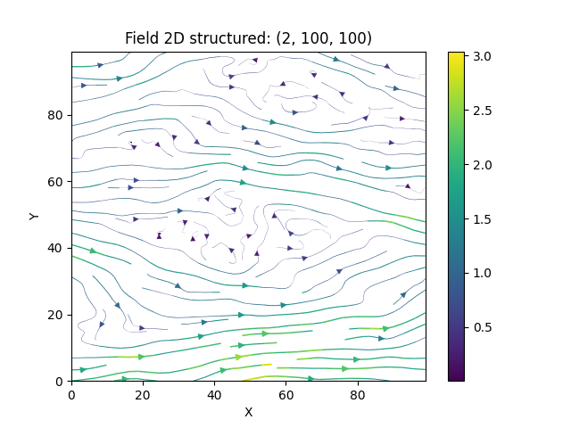
and we see, that the wiggles are much “rougher” than the smooth Gaussian ones.

Applications

One great advantage of the Kraichnan method is, that after some initializations, one can compute the velocity field at arbitrary points, online, with hardly any overhead. This means, that for a Lagrangian transport simulation for example, the velocity can be evaluated at each particle position very efficiently and without any interpolation. These field interpolations are a common problem for Lagrangian methods.