Note
Go to the end to download the full example code
Log-Normal Kriging
Log Normal kriging is a term to describe a special workflow for kriging to deal with log-normal data, like conductivity or transmissivity in hydrogeology.
It simply means to first convert the input data to a normal distribution, i.e. applying a logarithic function, then interpolating these values with kriging and transforming the result back with the exponential function.
The resulting kriging variance describes the error variance of the log-values of the target variable.
In this example we will use ordinary kriging.
import numpy as np

import gstools as gs

# condtions
cond_pos = [0.3, 1.9, 1.1, 3.3, 4.7]
cond_val = [0.47, 0.56, 0.74, 1.47, 1.74]
# resulting grid
gridx = np.linspace(0.0, 15.0, 151)
# stable covariance model
model = gs.Stable(dim=1, var=0.5, len_scale=2.56, alpha=1.9)
In order to result in log-normal kriging, we will use the LogNormal
Normalizer. This is a parameter-less normalizer, so we don’t have to fit it.
normalizer = gs.normalizer.LogNormal
Now we generate the interpolated field as well as the mean field.
This can be done by setting only_mean=True in Krige.__call__.
The result is then stored as mean_field.
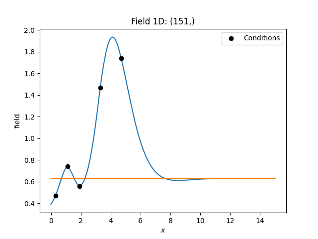
In terms of log-normal kriging, this mean represents the geometric mean of the field.
krige = gs.krige.Ordinary(model, cond_pos, cond_val, normalizer=normalizer)
# interpolate the field
krige(gridx)
# also generate the mean field
krige(gridx, only_mean=True)
And that’s it. Let’s have a look at the results.
ax = krige.plot()
# plotting the geometric mean
krige.plot("mean_field", ax=ax)
# plotting the conditioning data
ax.scatter(cond_pos, cond_val, color="k", zorder=10, label="Conditions")
ax.legend()

Total running time of the script: ( 0 minutes 0.172 seconds)