Note
Go to the end to download the full example code.
Kriging geographical data
In this example we are going to interpolate actual temperature data from the German weather service DWD.
Data is retrieved utilizing the beautiful package wetterdienst, which serves as an API for the DWD data.
For better visualization, we also download a simple shapefile of the German borderline with cartopy.
In order to keep the number of dependecies low, the calls of both functions shown beneath are commented out.
import matplotlib.pyplot as plt
import numpy as np

import gstools as gs


def get_borders_germany():
    """Download simple german shape file with cartopy."""
    import geopandas as gp  # 0.8.1
    from cartopy.io import shapereader as shp_read  # version 0.18.0

    shpfile = shp_read.natural_earth("50m", "cultural", "admin_0_countries")
    df = gp.read_file(shpfile)  # only use the simplest polygon
    poly = df.loc[df["ADMIN"] == "Germany"]["geometry"].values[0][0]
    np.savetxt("de_borders.txt", list(poly.exterior.coords))


def get_dwd_temperature(date="2020-06-09 12:00:00"):
    """Get air temperature from german weather stations from 9.6.20 12:00."""
    from wetterdienst.dwd import observations as obs  # version 0.13.0

    settings = dict(
        resolution=obs.DWDObservationResolution.HOURLY,
        start_date=date,
        end_date=date,
    )
    sites = obs.DWDObservationStations(
        parameter_set=obs.DWDObservationParameterSet.TEMPERATURE_AIR,
        period=obs.DWDObservationPeriod.RECENT,
        **settings,
    )
    ids, lat, lon = sites.all().loc[:, ["STATION_ID", "LAT", "LON"]].values.T
    observations = obs.DWDObservationData(
        station_ids=ids,
        parameters=obs.DWDObservationParameter.HOURLY.TEMPERATURE_AIR_200,
        periods=obs.DWDObservationPeriod.RECENT,
        **settings,
    )
    temp = observations.all().VALUE.values
    sel = np.isfinite(temp)
    # select only valid temperature data
    ids, lat, lon, temp = ids.astype(float)[sel], lat[sel], lon[sel], temp[sel]
    head = "id, lat, lon, temp"  # add a header to the file
    np.savetxt("temp_obs.txt", np.array([ids, lat, lon, temp]).T, header=head)
If you want to download the data again, uncomment the two following lines. We will simply load the resulting files to gain the border polygon and the observed temperature along with the station locations given by lat-lon values.
# get_borders_germany()
# get_dwd_temperature(date="2020-06-09 12:00:00")

border = np.loadtxt("de_borders.txt")
ids, lat, lon, temp = np.loadtxt("temp_obs.txt").T
First we will estimate the variogram of our temperature data. As the maximal bin distance we choose 900 km.
bin_center, vario = gs.vario_estimate(
    (lat, lon), temp, latlon=True, geo_scale=gs.KM_SCALE, max_dist=900
)
Now we can use this estimated variogram to fit a model to it.
Here we will use a Spherical model. We select the latlon option
to use the Yadrenko variant of the model to gain a valid model for lat-lon
coordinates and we set the geo_scale to the earth-radius. Otherwise the length
scale would be given in radians representing the great-circle distance.
We deselect the nugget from fitting and plot the result afterwards.
Note
You need to plot the Yadrenko variogram, since the standard variogram still holds the ordinary routine that is not respecting the great-circle distance.
model = gs.Spherical(latlon=True, geo_scale=gs.KM_SCALE)
model.fit_variogram(bin_center, vario, nugget=False)
ax = model.plot("vario_yadrenko", x_max=max(bin_center))
ax.scatter(bin_center, vario)
print(model)
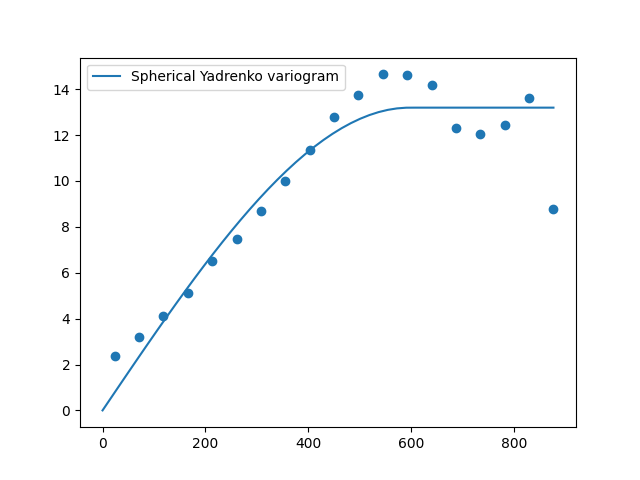
Spherical(latlon=True, var=13.2, len_scale=5.96e+02, geo_scale=6.37e+03)
As we see, we have a rather large correlation length of 600 km.
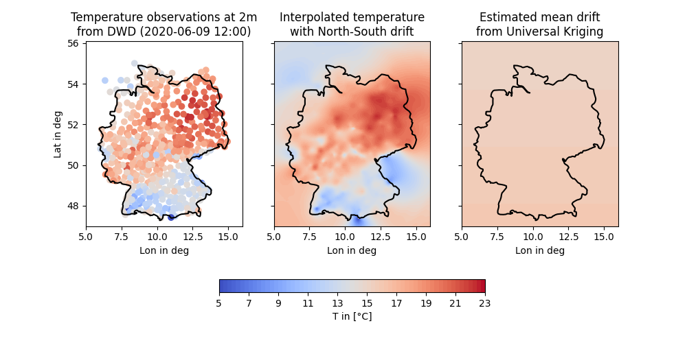
Now we want to interpolate the data using Universal kriging.
In order to tinker around with the data, we will use a north-south drift
by assuming a linear correlation with the latitude.
This can be done as follows:
Now we generate the kriging field, by defining a lat-lon grid that covers
the whole of Germany. The Krige class provides the option to only
krige the mean field, so one can have a glimpse at the estimated drift.
And that’s it. Now let’s have a look at the generated field and the input data along with the estimated mean:
levels = np.linspace(5, 23, 64)
fig, ax = plt.subplots(1, 3, figsize=[10, 5], sharey=True)
sca = ax[0].scatter(lon, lat, c=temp, vmin=5, vmax=23, cmap="coolwarm")
co1 = ax[1].contourf(g_lon, g_lat, uk["temp_field"], levels, cmap="coolwarm")
co2 = ax[2].contourf(g_lon, g_lat, uk["mean_field"], levels, cmap="coolwarm")

[ax[i].plot(border[:, 0], border[:, 1], color="k") for i in range(3)]
[ax[i].set_xlim([5, 16]) for i in range(3)]
[ax[i].set_xlabel("Lon in deg") for i in range(3)]
ax[0].set_ylabel("Lat in deg")

ax[0].set_title("Temperature observations at 2m\nfrom DWD (2020-06-09 12:00)")
ax[1].set_title("Interpolated temperature\nwith North-South drift")
ax[2].set_title("Estimated mean drift\nfrom Universal Kriging")

fmt = dict(orientation="horizontal", shrink=0.5, fraction=0.1, pad=0.2)
fig.colorbar(co2, ax=ax, **fmt).set_label("T in [°C]")
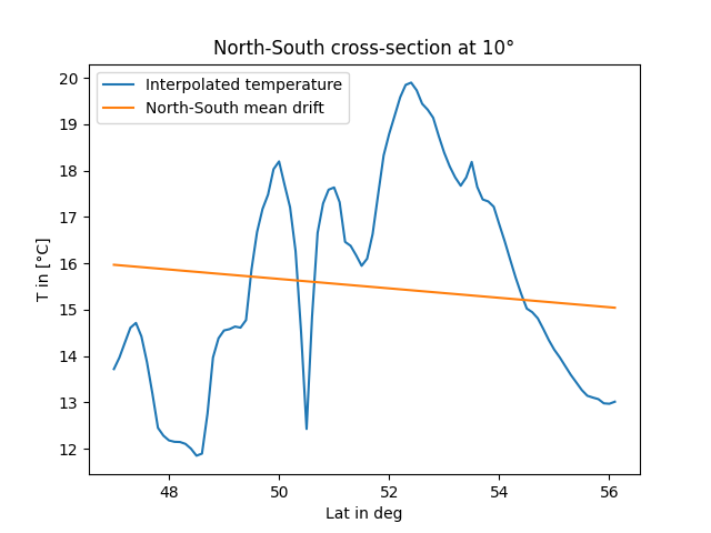
To get a better impression of the estimated north-south drift, we’ll take a look at a cross-section at a longitude of 10 degree:
fig, ax = plt.subplots()
ax.plot(g_lat, uk["temp_field"][:, 50], label="Interpolated temperature")
ax.plot(g_lat, uk["mean_field"][:, 50], label="North-South mean drift")
ax.set_xlabel("Lat in deg")
ax.set_ylabel("T in [°C]")
ax.set_title("North-South cross-section at 10°")
ax.legend()
Interpretion of the results is now up to you! ;-)
Total running time of the script: (0 minutes 4.860 seconds)