Note
Go to the end to download the full example code.
Directional variogram estimation and fitting in 3D
In this example, we demonstrate how to estimate a directional variogram by setting the estimation directions in 3D.
Afterwards we will fit a model to this estimated variogram and show the result.
import matplotlib.pyplot as plt
import numpy as np
from mpl_toolkits.mplot3d import Axes3D

import gstools as gs
Generating synthetic field with anisotropy and rotation by Tait-Bryan angles.
dim = 3
# rotation around z, y, x
angles = [np.deg2rad(90), np.deg2rad(45), np.deg2rad(22.5)]
model = gs.Gaussian(dim=3, len_scale=[16, 8, 4], angles=angles)
x = y = z = range(50)
pos = (x, y, z)
srf = gs.SRF(model, seed=1001)
field = srf.structured(pos)
Here we generate the axes of the rotated coordinate system to get an impression what the rotation angles do.
Now we estimate the variogram along the main axes. When the main axes are unknown, one would need to sample multiple directions and look for the one with the longest correlation length (flattest gradient). Then check the transversal directions and so on.
bin_center, dir_vario, counts = gs.vario_estimate(
    pos,
    field,
    direction=main_axes,
    bandwidth=10,
    sampling_size=2000,
    sampling_seed=1001,
    mesh_type="structured",
    return_counts=True,
)
Afterwards we can use the estimated variogram to fit a model to it. Note, that the rotation angles need to be set beforehand.
print("Original:")
print(model)
model.fit_variogram(bin_center, dir_vario)
print("Fitted:")
print(model)
Original:
Gaussian(dim=3, var=1.0, len_scale=16.0, anis=[0.5, 0.25], angles=[1.57, 0.785, 0.393])
Fitted:
Gaussian(dim=3, var=0.972, len_scale=13.0, nugget=0.0138, anis=[0.542, 0.281], angles=[1.57, 0.785, 0.393])
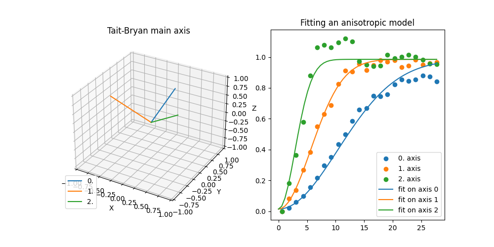
Plotting main axes and the fitted directional variogram.
fig = plt.figure(figsize=[10, 5])
ax1 = fig.add_subplot(121, projection=Axes3D.name)
ax2 = fig.add_subplot(122)

ax1.plot([0, axis1[0]], [0, axis1[1]], [0, axis1[2]], label="0.")
ax1.plot([0, axis2[0]], [0, axis2[1]], [0, axis2[2]], label="1.")
ax1.plot([0, axis3[0]], [0, axis3[1]], [0, axis3[2]], label="2.")
ax1.set_xlim(-1, 1)
ax1.set_ylim(-1, 1)
ax1.set_zlim(-1, 1)
ax1.set_xlabel("X")
ax1.set_ylabel("Y")
ax1.set_zlabel("Z")
ax1.set_title("Tait-Bryan main axis")
ax1.legend(loc="lower left")

x_max = max(bin_center)
ax2.scatter(bin_center, dir_vario[0], label="0. axis")
ax2.scatter(bin_center, dir_vario[1], label="1. axis")
ax2.scatter(bin_center, dir_vario[2], label="2. axis")
model.plot("vario_axis", axis=0, ax=ax2, x_max=x_max, label="fit on axis 0")
model.plot("vario_axis", axis=1, ax=ax2, x_max=x_max, label="fit on axis 1")
model.plot("vario_axis", axis=2, ax=ax2, x_max=x_max, label="fit on axis 2")
ax2.set_title("Fitting an anisotropic model")
ax2.legend()

plt.show()
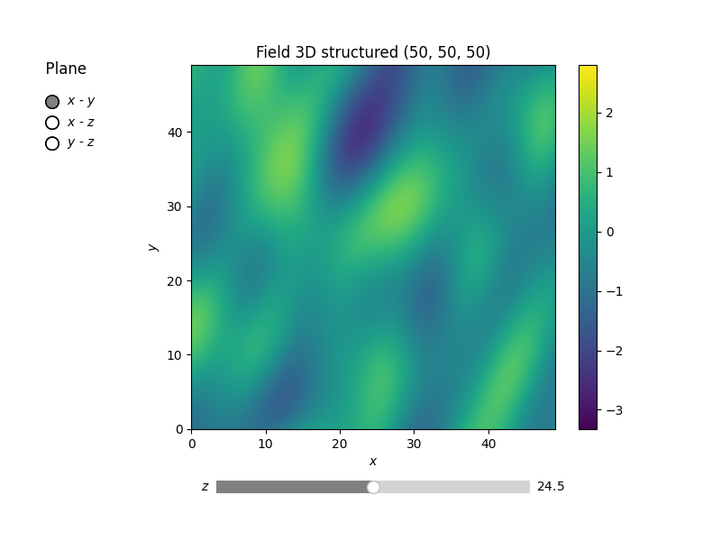
Also, let’s have a look at the field.
srf.plot()
Total running time of the script: (0 minutes 4.482 seconds)