Note
Go to the end to download the full example code.
Creating a 1D Synthetic Precipitation Field
In this example we will create a time series of a 1D synthetic precipitation field.
We’ll start off by creating a Gaussian random field with an exponential variogram, which seems to reproduce the spatial correlations of precipitation fields quite well. We’ll create a daily timeseries over a one dimensional cross section of 50km. This workflow is suited for sub daily precipitation time series.
import copy

import matplotlib.pyplot as plt
import numpy as np

import gstools as gs

# fix the seed for reproducibility
seed = 20170521
# spatial axis of 50km with a resolution of 1km
x = np.arange(0, 50, 1.0)
# half daily timesteps over three months
t = np.arange(0.0, 90.0, 0.5)

# space-time anisotropy ratio given in units d / km
st_anis = 0.4

# an exponential variogram with a corr. lengths of 2d and 5km
model = gs.Exponential(
    temporal=True, spatial_dim=1, var=1, len_scale=5, anis=st_anis
)
# create a spatial random field instance
srf = gs.SRF(model, seed=seed)

pos, time = [x], [t]

# a Gaussian random field which is also saved internally for the transformations
srf.structured(pos + time)
P_gau = copy.deepcopy(srf.field)
Next, we could take care of the dry periods. Therefore we would simply introduce a lower threshold value. But we will combine this step with the next one. Anyway, for demonstration purposes, we will also do it with the threshold value now.
threshold = 0.85
P_cut = copy.deepcopy(srf.field)
P_cut[P_cut <= threshold] = 0.0
With the above lines of code we have created a cut off Gaussian spatial random field with an exponential variogram. But precipitation fields are not distributed Gaussian. Thus, we will now transform the field with an inverse box-cox transformation (create a non-Gaussian field) , which is often used to account for the skewness of precipitation fields. Different values have been suggested for the transformation parameter lambda, but we will stick to 1/2. As already mentioned, we will perform the cutoff for the dry periods with this transformation implicitly with the shift. The warning will tell you that values have indeed been cut off and it can be ignored. We call the resulting field Gaussian anamorphosis.
# the lower this value, the more will be cut off, a value of 0.2 cuts off
# nearly everything in this example.
cutoff = 0.55
gs.transform.boxcox(srf, lmbda=0.5, shift=-1.0 / cutoff)
/home/docs/checkouts/readthedocs.org/user_builds/gstools/envs/stable/lib/python3.11/site-packages/gstools/transform/array.py:137: UserWarning: Box-Cox: Some values will be cut off!
  warn("Box-Cox: Some values will be cut off!")
As a last step, the amount of precipitation is set. This should of course be calibrated towards observations (the same goes for the threshold, the variance, correlation length, and so on).
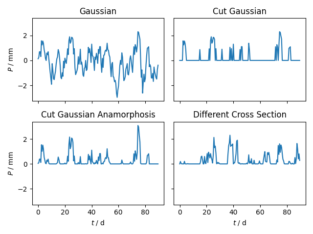
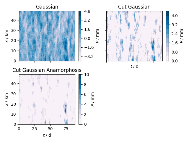
Finally we can have a look at the fields resulting from each step. Note, that the cutoff of the cut Gaussian only approximates the cutoff values from the box-cox transformation. For a closer look, we will examine a cross section at an arbitrary location. And afterwards we will create a contour plot for visual candy.
fig, axs = plt.subplots(2, 2, sharex=True, sharey=True)

axs[0, 0].set_title("Gaussian")
axs[0, 0].plot(t, P_gau[20, :])
axs[0, 0].set_ylabel(r"$P$ / mm")

axs[0, 1].set_title("Cut Gaussian")
axs[0, 1].plot(t, P_cut[20, :])

axs[1, 0].set_title("Cut Gaussian Anamorphosis")
axs[1, 0].plot(t, P_ana[20, :])
axs[1, 0].set_xlabel(r"$t$ / d")
axs[1, 0].set_ylabel(r"$P$ / mm")

axs[1, 1].set_title("Different Cross Section")
axs[1, 1].plot(t, P_ana[10, :])
axs[1, 1].set_xlabel(r"$t$ / d")

plt.tight_layout()

fig, axs = plt.subplots(2, 2, sharex=True, sharey=True)

axs[0, 0].set_title("Gaussian")
cont = axs[0, 0].contourf(t, x, P_gau, cmap="PuBu", levels=10)
cbar = fig.colorbar(cont, ax=axs[0, 0])
cbar.ax.set_ylabel(r"$P$ / mm")
axs[0, 0].set_ylabel(r"$x$ / km")

axs[0, 1].set_title("Cut Gaussian")
cont = axs[0, 1].contourf(t, x, P_cut, cmap="PuBu", levels=10)
cbar = fig.colorbar(cont, ax=axs[0, 1])
cbar.ax.set_ylabel(r"$P$ / mm")
axs[0, 1].set_xlabel(r"$t$ / d")

axs[1, 0].set_title("Cut Gaussian Anamorphosis")
cont = axs[1, 0].contourf(t, x, P_ana, cmap="PuBu", levels=10)
cbar = fig.colorbar(cont, ax=axs[1, 0])
cbar.ax.set_ylabel(r"$P$ / mm")
axs[1, 0].set_xlabel(r"$t$ / d")
axs[1, 0].set_ylabel(r"$x$ / km")

fig.delaxes(axs[1, 1])
plt.tight_layout()
Total running time of the script: (0 minutes 0.650 seconds)