Interface to PyKrige

To use fancier methods like regression kriging, we provide an interface to PyKrige (>v1.5), which means you can pass a GSTools covariance model to the kriging routines of PyKrige.

To demonstrate the general workflow, we compare ordinary kriging of PyKrige with the corresponding GSTools routine in 2D:

import numpy as np
from matplotlib import pyplot as plt
from pykrige.ok import OrdinaryKriging

import gstools as gs

# conditioning data
cond_x = [0.3, 1.9, 1.1, 3.3, 4.7]
cond_y = [1.2, 0.6, 3.2, 4.4, 3.8]
cond_val = [0.47, 0.56, 0.74, 1.47, 1.74]

# grid definition for output field
gridx = np.arange(0.0, 5.5, 0.1)
gridy = np.arange(0.0, 6.5, 0.1)

A GSTools based Gaussian covariance model:

model = gs.Gaussian(
    dim=2, len_scale=1, anis=0.2, angles=-0.5, var=0.5, nugget=0.1
)

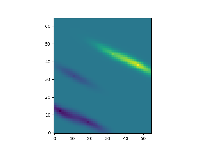
Ordinary Kriging with PyKrige

One can pass the defined GSTools model as variogram model, which will not be fitted to the given data. By providing the GSTools model, rotation and anisotropy are also automatically defined:

OK1 = OrdinaryKriging(cond_x, cond_y, cond_val, variogram_model=model)
z1, ss1 = OK1.execute("grid", gridx, gridy)
plt.imshow(z1, origin="lower")
plt.show()

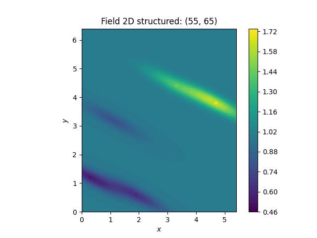
Ordinary Kriging with GSTools

The Ordinary kriging class is provided by GSTools as a shortcut to define ordinary kriging with the general Krige class.

PyKrige’s routines are using exact kriging by default (when given a nugget). To reproduce this behavior in GSTools, we have to set exact=True.

OK2 = gs.krige.Ordinary(model, [cond_x, cond_y], cond_val, exact=True)
OK2.structured([gridx, gridy])
ax = OK2.plot()
ax.set_aspect("equal")